Spaceship Titanic & Decision Trees

“The year is 2912, and interstellar travel is picking up speed. The Spaceship Titanic embarked on it’s maiden voyage a month ago, and sadly met the same fate as it’s namesake from 1,000 year ago. Although the ship is intact, about half the passengers have been transported to another dimension.

To help rescue crews and retrieve the lost passengers, you are challenged to predict which passengers were transported using records recovered from the spaceship’s damaged computer system.”

Such read the prompt of my first kaggle project. I had just finished an introductory machine learning course and was eager to get my hands dirty. I collaborated with a friend and we decided to tackle this problem, with our own twist. We would implement the algorithm required from scratch ! This post is an explanation of our project.

Part 1 : Exploring the Data

The dataset provided contains 13 columns that capture all the details (some relevant & others not) of the passengers on board, ranging from their PassengerId to how much money they spent at the FoodCourt.

Finding the total number of records (8,693) and their statistical features is routine, but reveals that the FoodCourt is the most used amenity, with the ShoppingMall on the opposite end. There are also large standard deviations, which imply that a few people dictate the trends. Next, we wanted to see how many records were missing.

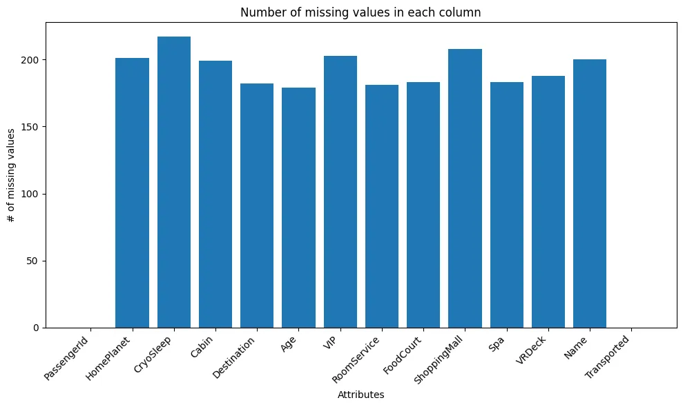Which values are missing, and how many ?

The first and last column have no missing values by design. Almost all columns beside have ~ 200 values missing, totaling ~2,000 values (25% of the data) ! We tried to drop the values but realized that they were independent, since we couldn’t loose a quarter of our values we had to find another way.

We used linear interpolation to fill in the missing values. Imagine you have two rows X and Z, where the values of FoodCourt are missing and you wish to find the missing value of FoodCourt at a row Y in between X and Z. We make a straight line connecting X and Z, and predict the value of Y based on it’s relative position to the line. The statistical features were largely unchanged after this process, a positive sign. With all the data in place, we moved on to learn some more.

Correlation measures whether two quantities are related linearly, i.e. does an increase in X corresponds to an increase in Y ? Finding the correlation between the columns can shed some light into transportation trends. A score of +1 means that increase in X corresponds to increase in Y, whereas -1 means that increase in X corresponds to decrease in Y.

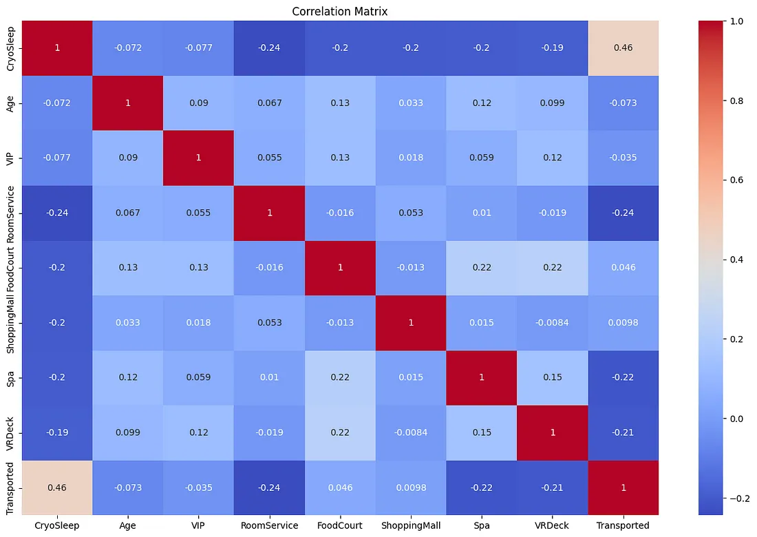What are the relations between variables ?

This reveals that Transported and Cryosleep are positively related. Since people in Cyrosleep are confined to their cabins, this means that people in their cabins are more likely to be transported than people on deck. RoomService, Spa and VRDeck are negatively related to Transported. This means that a person spending less on amenities is more like to be transported. This agrees with the previous result.

Next we wanted to see which planet most people departing are coming from as well as how many people in total were transported. This did not reveal much beside the fact that most people arrive from Earth and ~50% of the people onboard vanished. The resulting plots are shown below.

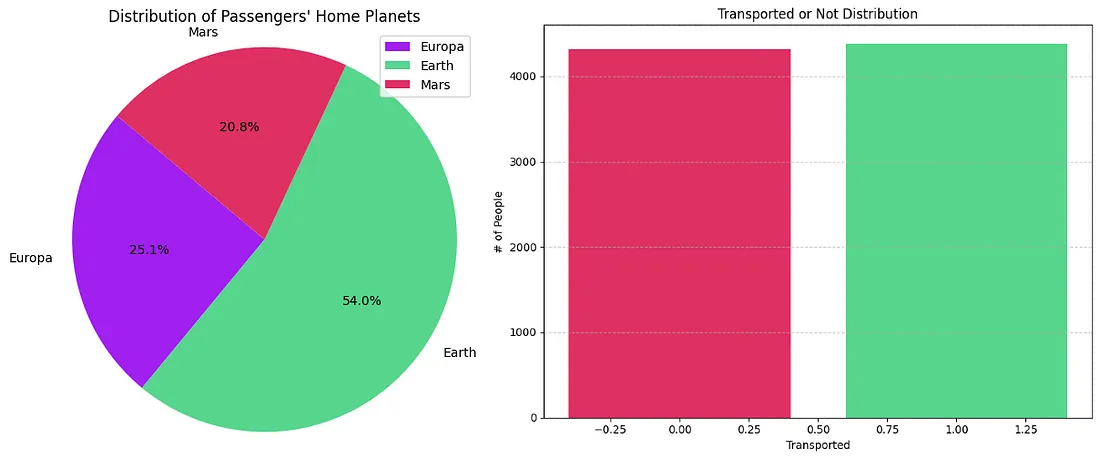Some basic passenger distributions

Something far more interesting is finding out the locations of the people who were actually distributed. This can be done by finding the rows (people) where Transported takes on a True value and then extracting the HomePlanet and Destination.

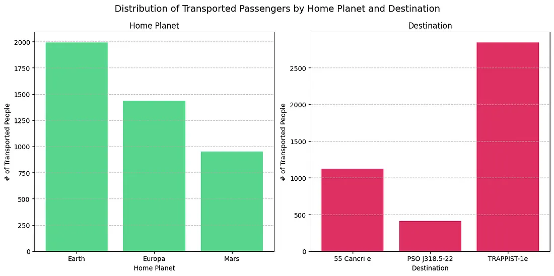Where were the missing people coming from, & where were they going ?

The majority of people transported were coming from Earth 😅 and headed to TRAPPIST-1e (may or may not have originated from Earth). This is an interesting trend, and could maybe help the model. It’s also a good idea to check if the same pattern is preserved once we make our predictions.

This brings us to the end of the data analysis. Now on to the fun part..

Part 2 : Decision Trees from Scratch

This image was generated using Meta AI

Imagine a large tree starting with a trunk, splitting into branches and these branches splitting into further branches. Decision Trees are very similar and are made up of multi layered, nested-if statements (conditions). And like a real tree, a Decision Tree also ends with leaves.

At each branch (node) the algorithm decides how to best split the data in order to optimize a few values. Once a condition is arrived at, the data is split accordingly into more nodes and the process starts anew on each sub tree. The node at which the splitting occurs is a parent node, and the splits created are called children nodes.

It is a machine learning algorithm because it comes up with the features to be used for splitting and their threshold values (yes, by itself) based on the data provided. The hope is that once a data point arrives at a leaf node, it has to be of a certain type (True or False, Koala Bear or Chimpanzee, ..)

Once a Decision Tree is built, new data, on which predictions are to be made is fed to it as data points. Each data point now goes down the Decision Tree based on the conditions until it reaches a leaf node. Finally a prediction of the data for that data point is made !

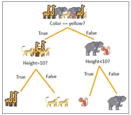
For example, a Decision Tree classifying animals is shown below. All the animals start out at the top and follow the conditions one by one till they reach a leaf node. We have now successfully built our tree. It is capable of classifying animals based on their color and height. To check it’s working we can use another animal (It’s funny to see that an shark would be classified as a monkey by this tree).

There are 2 mathematical formulae that govern the working of a Decision Tree, it is through these that the computer derives the features and their threshold values.

Entropy measures the non-uniformity of data at a particular node, for example the node with all the animals has high entropy. Here p represents the probability of a certain type (class) at a specific node, for example p(giraffe) = 3/8 at the start. Information gain measures the decrease in entropy between branch splits (parent and children nodes), w represents the appropriate weight (relative size).

At every node a Decision Tree minimizes the Entropy and maximizes the Information Gain. Now that we have the mathematics out of the way, we can continue to actual structure of the Decision Tree.

The structure of our Decision Tree

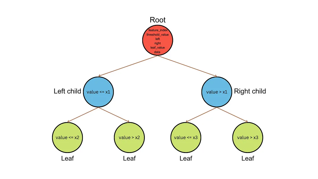
Our Decision Tree is made up of a custom Node class, these are the building blocks. Each Node has the following features

• feature_index: This attribute stores the index of the feature used to split the data at this node. It’s None for leaf nodes (where no further splitting occurs).
• threshold_value: This attribute stores the specific value of the feature used for splitting at this node. It’s None for leaf nodes.
• left: This attribute is the left child node of the current node. It’s None if the current node is a leaf node.
• right: This attribute is the right child node of the current node. It’s None if the current node is a leaf node.
• leaf_value: This attribute stores the majority class label of the data contained in this leaf node. It’s None for non-leaf nodes.
• data: This attribute can store the actual data points (rows) that belong to this node during the tree building process

Now that we have a Node class defined, we can work on building the Decision Tree. To do this we will be needing a few functions that implement all the logic and build our Decision Tree.

• split - Takes a dataset, feature index, and threshold value, and splits the data into left and right child datasets based on the threshold value.
• best_split - Iterates through all features and their possible values, finding the split that results in the maximum information gain.
• calculate_leaf_value - Calculates the majority class (most frequent target value) within a dataset, used for assigning a class label to leaf nodes.
• build_tree - Recursively builds the decision tree. It checks if the stopping criteria (depth or minimum samples) are met. If not, it finds the best split, creates a node with that information, splits the data, and recursively builds the left and right subtrees. Otherwise, it creates a leaf node with the majority class.
• fit - Takes the training data (X) and calls the build_tree function to construct the decision tree based on that data.
• predict_single - Takes a single data row and the current tree node. It recursively traverses the tree based on the feature values in the row until a leaf node is reached. The leaf node’s value (predicted class label) is returned.
• predict - Takes the entire testing data (Y) and calls predict_single for each row, building a list of predicted target values for all data points. This is the output that’s returned.

All that’s left to do is to implement the mathematical formulae in code. That is, we go over all possible values, for each column and check the resulting information gain. Then the data is split into appropriate nodes. This is done until we reach a stopping criterion, which is either minimum # of data points or maximum # of splits.

Once a model is trained on this data, we test it on new data. We feed the decision tree a data point, follow it down a leaf and return the majority class type for that leaf. This is the prediction of what that data point is. And there you have it, a Decision Tree from scratch ! The video tutorial I followed to understand Decision Trees can be found here.

Once we had our Decision Tree class in place, we fit (trained) the model and made our prediction. This resulted in a kaggle score of 0.75. We also wanted to compare our model against sklearn’s DecisionTreeRegressor, and to our surprise we outperformed it by 0.05 accuracy points :D

The entire source code of the project, along with the data can be found here.