Neural Networks from scratch
A neural network built from the ground up to solve digit recognition. I motivate theory and follow it up with code implementations. An in depth study of the 4 equations of backpropagation is provided at the end.
Making predictions
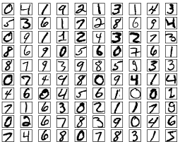
Identifying these images is a trivial task for humans. But just imagine trying to write a program to make a computer do the same, the many rules you would need to define: “A 9 has a loop and a straight line below it”, “Two loops on top of each other make an eight”, … and the list goes on and on
And this is just for 9 digits. Imagine the complexity of rule-based system for self-driving cars!
The classical machine learning algorithms we have seen so far, from Linear Regression till Support Vector Machines have been interpretable. And while they are machine learning in the sense that they get better with data, superior performance is found by hand-crafting features and rules, turning knobs and dials based on human knowledge. They are also limited in the types of problems they solve.
Neural networks are based on a completely different type of learning algorithm. We completely do away with rules and interpretability, trading it in for an unbiased system that can learn any complicated function out there. The drawback being that it requires large data & compute, explaining why neural networks only gained traction from the 2000s while the algorithms were developed all they way back in 1980.
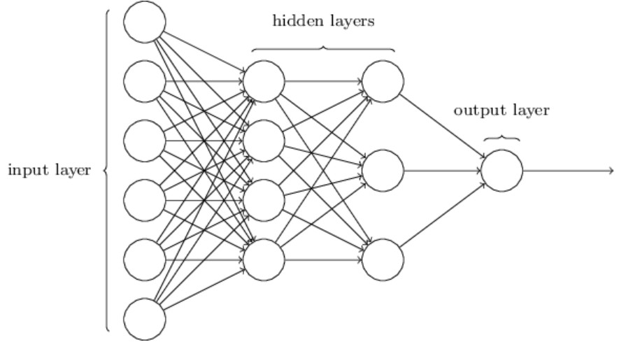
At the end of the day, we can think of a neural network as a function. One take takes in an input and spits out an output. A basic neural network has an input layer, some hidden layers and a final output layer. Each of these layers is made up of neurons, each neuron stores a number and is connected to all other neurons in the next layer. The final prediction we make, is related to the neurons in the final layer. An example neural network is shown below:
 Source: Michael Nielsen
Each connection between neurons carries a weight, emphasizing how important that neuron is to the one in question. Each neuron also has a bias, a threshold that makes the prediction more robust. Let’s image an overly simple neural network and see how we might use it to predict the rain:
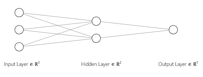
Suppose we take as input the vector $x = [x_1, x_2, x_3]$ representing the following features:
- $x_1$: moisture
- $x_2$: temperature
- $x_3$: wind speed
We pass this input into two neurons in the first layer:
-
The first neuron computes: \(y_1 = w_1 x + b_1 = w_{11}x_1 + w_{12}x_2 + w_{13}x_3 + b_1\) This might represent how close the air is to condensation.
-
The second neuron computes: \(y_2 = w_2 x + b_2 = w_{21}x_1 + w_{22}x_2 + w_{23}x_3 + b_2\) This could represent how windy and hot it is.
We then feed these two outputs into a third neuron in the next layer, which computes: \(z_1 = w_3 y_1 + w_4 y_2 + b_3\) This final output might represent the total chance of rain. If $z_1$ exceeds a certain threshold, the network predicts rain.
Now, since all operations are linear (no activation functions), the final output $z_1$ is still a linear function of the input $x$:
\[z_1 = w_3(w_1 x + b_1) + w_4(w_2 x + b_2) + b_3 \\ = (w_3 w_1 + w_4 w_2)x + (w_3 b_1 + w_4 b_2 + b_3) \\ = w x + b\]So ultimately, the entire network reduces to a single linear transformation of the input: \(z_1 = w x + b\)
A bunch of linear functions, can only approximate a linear function.This idea is explained beautifully in this short video by Emergent Garden. However, most relationships between input and output tend to be non-linear. And so we introduce a non-linearity. The final output of each neuron, is therefore made to be $\sigma(w \cdot x + b)$, where $\sigma$ is the non-linear function.
 Some of the most popular activation functions.
We will stick to the sigmoid “squishification” function. Coding it up is straightfoward, and we store it’s derivative too, for reasons we will see soon.
def sigmoid(z):
    return 1 / (1+exp(-z))

def sigmoid_prime(z):
    return sigmoid(z) * (1 - sigmoid(z))
Modern neural networks are built on a few powerful ideas:
-
Multiple neurons, each performing a simple computation.
-
Successive layers, where the output of one becomes the input of the next.
-
Non-linear activation functions, applied at each step.
Individually, each neuron is quite simple — it takes in a few numbers, multiplies them by weights, adds a bias, and (optionally) applies a non-linear function like a sigmoid or ReLU. But when you connect these neurons together in layers, and stack the layers into a deep network, something remarkable happens.
Through this structure, the network begins to build up complex behavior from simple parts. Early layers might detect basic patterns or relationships in the data. Later layers combine those patterns into more abstract concepts. The result is a system that can approximate highly non-linear functions — from recognizing handwriting to predicting the weather.
This entire architecture, where information flows in one direction — from input to output — without looping back, is known as a feedforward neural network. It’s a foundational model in deep learning, and a beautiful example of how simple components, carefully combined, can produce intelligent behavior.
def feedforward(self,a):
  for w,b in zip(self.weights, self.biases):
    a = sigmoid(np.dot(w,a) +b) # Recursively computes activations for each layer and "feeds-forward" ; use a1 as input for layer 2, and so on
  return a
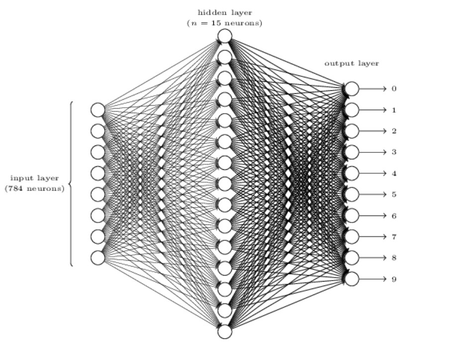
In our problem of digit classification, we accept 28x28 images as individual images in pixel form, for a total of 784 input neurons. The final layer then, has 10 neurons, one for each digit. The neuron with the highest activation, is our prediction for the digit. An example network may look like the following:
 Source: Michael Nielsen
🚨 This section had sloppy mathematics and hand-wavy notation. The point was purely illustrative, and the mathematics involved is clearly articulated later in the article.
How will it learn?
Every good machine learning algorithm needs a cost function, a way to quantify it’s performance, and get better. This cost function depends on a very large number of parameters. Finding out how these parameters influence the cost (and therefore the model’s performance) is the perineal problem of computer scientists. Here, the lower the cost the better.
Here, since we are trying to classify digits, classification accuracy could be a good choice right? Well … not exactly, we would like to impose two conditions on our cost function:
-
The cost function can be written as a function of the outputs of the network
-
The cost function is “smooth” or continuous, so that small changes in the input produce small changes in the output
With all these ideas in place, the mean squared error loss, is a good loss function.
\[L = \frac{1}{n} \sum_{i}^{n} (\hat{y}-y)^{2}\]Where $\hat{y}$ is the neural network’s prediction, and $y$ is the true label for that observation. So our output layer would have 10 neurons, and the neuron with highest activation would be our models’ prediction.
As discussed earlier, our model’s prediction is the neuron with the highest activation. But, how confident is it of that number? It is 70-30 or more like 51-49? The loss function will tell us exactly that, with a higher value indicating lower confidence. It measures the difference between the actual neuron activations and the expected, ideal neuron activations. Here, the ideal activations would be 1 for the number and 0 everywhere else, 100% certainty.
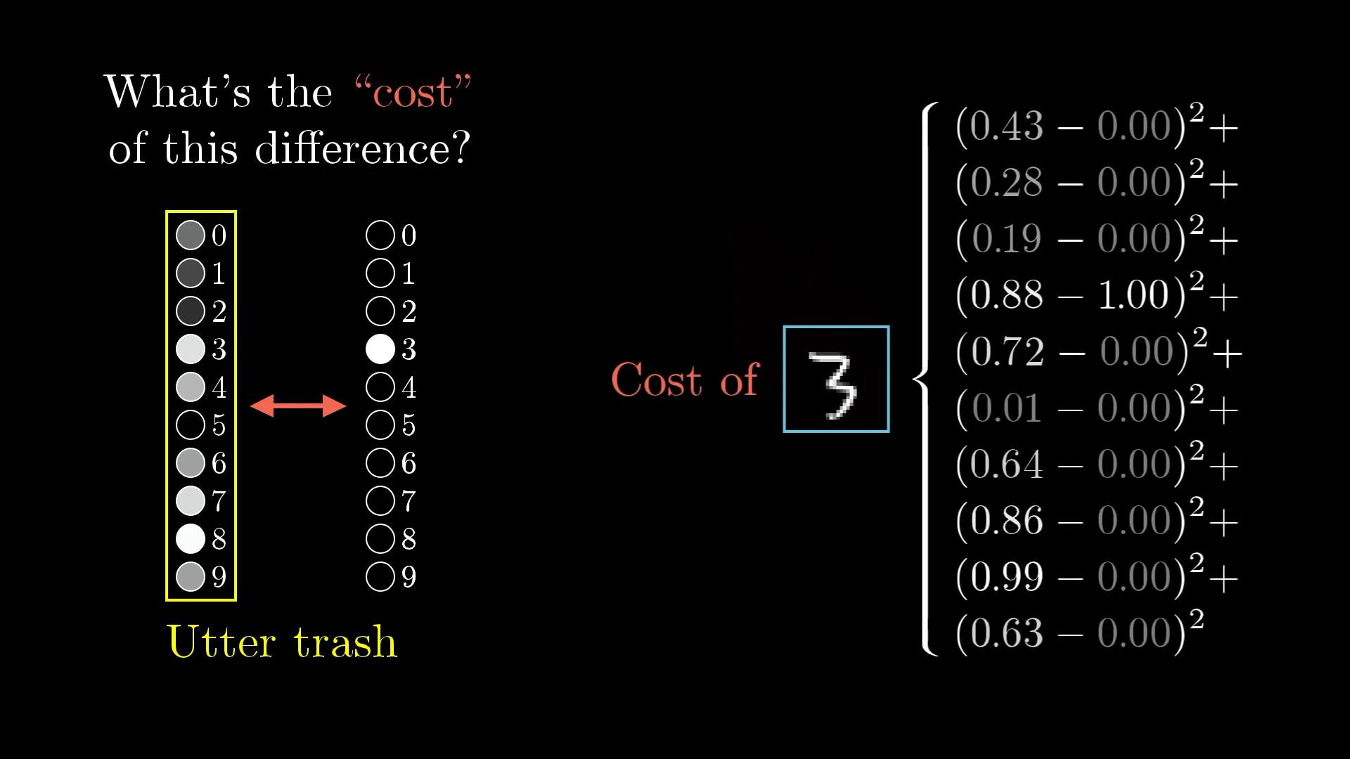 Source: 3Blue1Brown
We turn now to one optimizing or lowering the cost, indeed the most popular method used in Deep Learning, gradient decent. The idea is best visualized in 2-dimensions. Imagine that all the values that the cost function can take forms a mountain. This mountain has peaks and valleys, and we would like to end up at the lowest valley, reduce the cost as much as possible.
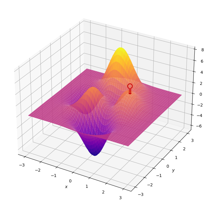
Imagine you are at a random point on this mountain, and you want to know the direction of your next step, the best step you could take. A step that decreases your height the most. Mathematical wizardry makes this possible. Th gradient of a function, denoted $\nabla C$ tells us the direction to step in, and also the size of our step. I will explain this with an example:
\[\nabla C = \begin{pmatrix} \color{Blue}{+2.00} \\ \color{Red}{-0.30} \end{pmatrix}\]Here each row represents one particular direction or dimension. The large positive magnitude indicates we need to take a big positive step in that direction. While the small negative magnitude indicated we need to take a small negative step in the other.
A little caveat, the gradient tells us the direction of steepest ascent. So we just walk the opposite way. Ah, we now have a simple update rule
\[x_{n+1} = x_{n} - \eta \nabla f_{x} \\ y_{n+1} = y_{n} - \eta \nabla f_{y}\]The factor eta ($\eta$) is called the learning rate, something that controls how quickly we converge (if we do) to a local minimum or valley.
A neural network is defined by it’s weights and biases, the dimensions of the cost function. Hence, in our case, the update rule looks like:
\[w_{n+1} = w_{n} - \nabla C_{w} \\ b_{n+1} = b_{n} - \nabla C_{b}\]Each training example would nudge the weights in a different direction, and if we changed them according to just one example, it would be good at predicting a single digit, say like a 9 or an 8. But we want our network to predict all digits better, and so we take an average gradient over all the examples we have seen. Wishing that the network does a better job at capturing all digits.
def update_mini_batch(self, mini_batch, eta):# Update the weight's and biases using average of gradients from each training example
        nabla_b = [np.zeros(b.shape) for b in self.biases]
        nabla_w = [np.zeros(w.shape) for w in self.weights]
        for (x,y) in mini_batch:
            delta_nabla_b, delta_nabla_w = self.backprop(x,y) # Gradients with respect to biases and weights for example (x,y)
            nabla_b = [nb+dnb for (nb,dnb) in zip(nabla_b, delta_nabla_b)] # Add up all the gradients from all the training examples
            nabla_w = [nw+dnw for (nw,dnw) in zip(nabla_w, delta_nabla_w)]
        self.weights = [w - (eta/len(mini_batch))*nw for (w,nw) in zip(self.weights, nabla_w)] # Subtract the average gradients
        self.biases = [b - (eta/len(mini_batch))*nb for (b,nb) in zip(self.biases, nabla_b)]
In practice, computing the (very high dimensional) gradient for every single training example then summing them updating the weights and biases turns out to be computationally expensive.
We now make one last assumption to help us:
- The cost function can be written as an average $C = \frac{1}{n} \sum_{x=1}^{n} C_{x}$ where $C_{x}$ is the cost per training example
We trade in preciseness for practicality, and get an answer that’s approximately right. Doing the training in such batches is called stochastic gradient decent, and is the norm for training Deep Learning methods.
def SGD(self, training_data, epochs, mini_batch_size, eta, test_data=None): # Train neural network using stochastic gradient descent
        if test_data: n_test = len(test_data)
        n = len(training_data)
        for j in range(epochs): # Repeat all the steps below for required number of epochs
            random.shuffle(training_data)
            mini_batches = [training_data[k:k+mini_batch_size] for k in range(0,n,mini_batch_size)] # Get splits of data in mini batch sizes
            for mini_batch in mini_batches:
                self.update_mini_batch(mini_batch, eta) # Update the weights and biases according to the average gradient of that mini batch
            if test_data:
                print(f"Epoch {j} accuracy: {self.evaluate(test_data)}/{n_test}")
            else:
                print(f"Epoch {j} complete")
Mathematical set up
Let’s start by discussing notation, like good math boys.
The weight connecting the $k^{th}$ neuron in layer $l$ to the $j^{th}$ neuron in layer $l-1$ is denoted by $w_{jk}^{l}$. The bias of the $j^{th}$ neuron in the $l^{th}$ layer is given by $b_{j}^{l}$. Similarly activation of the $j^{th}$ neuron in the $l^{th}$ layer is given by $a_{j}^{l}$
Phew that was a lot, let’s take a simple example and make sense of it. Assume a neural network with very many layers. For the time being we only care about layers 4 and 5 which are shown below
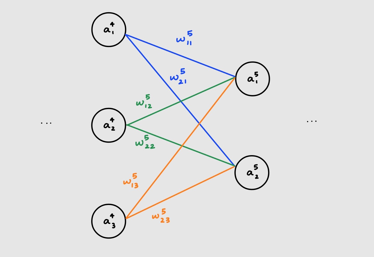
Let’s compute the activation at layer 5:
\[a_{1}^{5} = \sigma(\color{Blue}{w_{11}^{5}a_{1}^{4}} \hspace{2mm} \color{Black}{+} \hspace{2mm} \color{Green}{w_{12}^{5}a_{2}^{4}} \hspace{2mm} \color{Black}{+} \hspace{2mm} \color{Orange}{w_{13}^{5}a_{3}^{4}} \hspace{2mm} \color{Black}{+} \hspace{2mm} b_{1}^{5}) \\ \\ a_{2}^{5} = \sigma(\color{Blue}{w_{21}^{5}a_{1}^{4}} \hspace{2mm} \color{Black}{+} \hspace{2mm} \color{Green}{w_{22}^{5}a_{2}^{4}} \hspace{2mm} \color{Black}{+} \hspace{2mm} \color{Orange}{w_{23}^{5}a_{3}^{4}} \hspace{2mm} \color{Black}{+} \hspace{2mm} b_{2}^{5})\]Since these are linear equations (aside from the sigmoid) we can represent this using a matrix
\[\begin{pmatrix} a_{1}^{5} \\ a_{2}^{5} \end{pmatrix} = \sigma \left\{ \begin{pmatrix} \color{Blue}{w_{11}^{5}} & \color{Green}{w_{12}^{5}} & \color{Orange}{w_{13}^{5}}\\ \color{Blue}{w_{21}^{5}} & \color{Green}{w_{22}^{5}} & \color{Orange}{w_{23}^{5}} \end{pmatrix} \cdot \begin{pmatrix} \color{Blue}{a_{1}^{4}} \\ \color{Green}{a_{2}^{4}} \\ \color{Orange}{a_{3}^{4}} \end{pmatrix} + \begin{pmatrix} b_{1}^{5}\\ b_{2}^{5} \end{pmatrix} \right\}\]Ah, written this way it’s easy to see that the activation for neuron i is simply a sum of all the weights that lead to i times their corresponding activations. Plus an additional bias ofcourse.
$a_{j}^{l} = \sigma(\sum_{k} w_{jk}a_{k}^{l-1} + b_{j}^{l}) = \sigma(z_{j}^{l})$
Here $z_{j}^{l}$ is an intermediate variable representing the input that neuron $j$ at layer $l$ receives.
Notice that the number of rows = number of neurons in layer $l$ while the number of columns = number of neurons in layer $l-1$. Going across a row we find all the weights required for $a_{j}^{l}$ While going down a column $k$ tells us all the weights associated with $a_{k}^{l-1}$. Let’s also consider the transpose of this matrix.
\[(w^{5})^{T} = \begin{pmatrix} \color{Blue}{w_{11}^{5}} & \color{Blue}{w_{21}^{5}} \\ \color{Green}{w_{12}^{5}} & \color{Green}{w_{22}^{5}} \\ \color{Orange}{w_{13}^{5}} & \color{Orange}{w_{23}^{5}} \end{pmatrix}\]Here, Notice that the number of rows = number of neurons in layer $l-1$ while the number of columns = number of neurons in layer $l$. Going across a row we find all the weights required for $a_{j}^{l-1}$ While going down a column $k$ tells us all the weights associated with $a_{k}^{l}$. This gives us a way to go from $l+1 \to l$, a map for walking backwards.
With all the linear algebra in place, we define the basic structure of our neural network! We won’t be defining any individual neurons, since we only care about the weights and biases.
class Network():
    def __init__(self, sizes):
        self.num_layers = len(sizes)
        self.sizes = sizes # Example [2,3,1] means 2 neurons in first layer, 3 neurons in the hidden layer and 1 neuron in output layer
        self.biases = [np.random.randn(y,1) for y in sizes[1:]] # One bias vector per layer, example: [0.6,0.8,0.3] for layer #2
        self.weights = [np.random.randn(y,x) for x,y in zip(sizes[:-1], sizes[1:])] # One weight matrix per two hidden layers, example: [[.4,.6],[.1,.2],[.5..5]] for layer 2
Backpropagation under the hood
Now comes the scary calculus :’) The program of backpropagation is to understand how the cost function would change for small changes in individual weights and biases. With this information we can change the culprits responsible for sub-par performance.
Since, the weights and biases we need are all captured in $z_{j}^{l}$. We can first see how making a small change to the input to the neuron, $z_{j}^{l} + \color{Blue}{\Delta z_{j}^{l}}$ affects the final cost, then work our way back to catch the responsible weights and biases.
Therefore, we define the error of neuron $j$ at layer $l$ to be $\delta_{j}^{l} = \frac{\partial C}{\partial z_{j}^{l}}$. We will the use some calculus to derive $\frac{\partial C}{\partial w_{jk}^{l}}$ and $\frac{\partial C}{\partial b_{j}^{l}}$
Backpropogation relies heavily on the idea of the chain rule. Here is an intuitive explanation of the main idea: “If a car travels twice as fast as a bicycle and the bicycle is four times as fast as a walking man, then the car travels 2 × 4 = 8 times as fast as the man.” - George F. Simmons
Let’s collect everything we have seen so far, and how each part is connected to the rest. This helped me understand the entire process deeper, and was especially useful during the proofs.
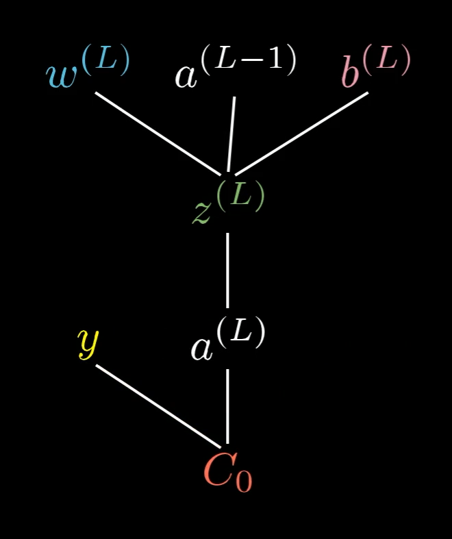 The many moving parts and their relations. Source: 3Blue1Brown
Without further ado, the four equations of backpropagation are:
\[\begin{equation} \delta_{j}^{L} = \frac{\partial C}{\partial a_{j}^{L}} \cdot \sigma'(z_{j}^{L}) \end{equation}\]The error in the output layer
We know how the cost relates to the final activation, and how the activation relates to it’s input. In particular:
$ C = \frac{1}{2} \parallel y - a_{j}^{L} \parallel^{2}$ where $a_{j}^{L}=\sigma(z_{j}^{L})$
Applying the chain rule we get that
$\frac{\partial C}{\partial z_{j}^{L}} = \frac{\partial C}{ \partial a_{j}^{L}} \cdot \frac{\partial a_{j}^{L}}{\partial z_{j}^{L}} = \frac{\partial C}{ \partial a_{j}^{L}} \cdot \sigma’(z_{j}^{L})$
\[\begin{equation} \delta_{j}^{l} = \sum_{k} w_{kj}^{l+1} \delta_{k}^{l+1} \cdot \sigma'(z_{j}^{l}) \end{equation}\]The error in layer $l$ as a function of the error in layer $l+1$
This is a little trickier. We need to think about how the error at layer $l$ propagates to the next layer. Let’s visualize what’s happening
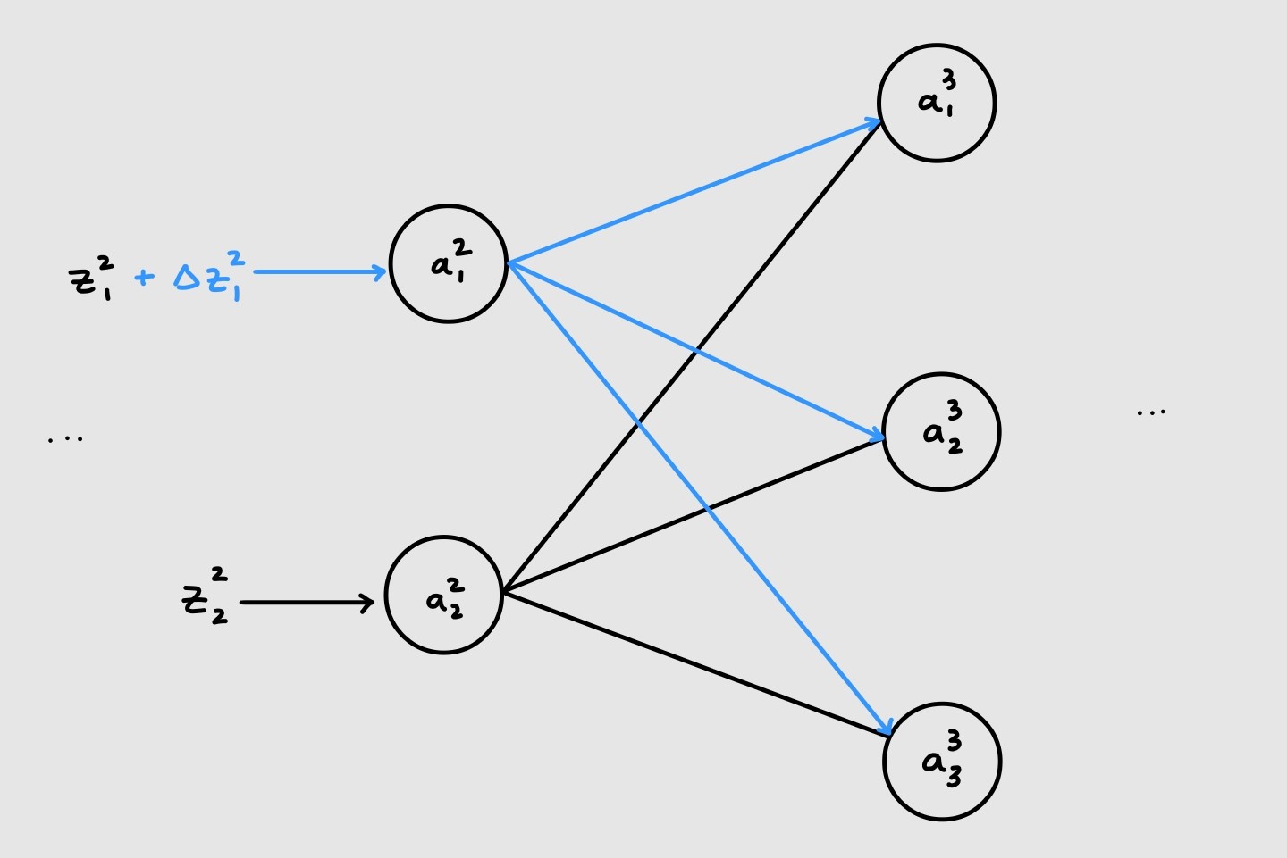
As can be seen above, the first neuron of the first layer is connected to all the neurons in the next layer. Hence, making a small change to it’s input will affect the inputs to all the neurons of the next layer.
Now, our task is to rewrite $\delta_{j}^{l}$ in terms of $\delta_{k}^{l+1}$. Using what we saw above,
$\delta_{j}^{l}= \frac{\partial C}{\partial z_{j}^{l}} = \sum_{k}\frac{\partial C}{\partial z_{k}^{l+1}} \cdot \frac{\partial z_{k}^{l+1}}{\partial z_{j}^{l}} = \sum_{k} \delta_{k}^{l+1} \cdot \frac{\partial z_{k}^{l+1}}{\partial z_{j}^{l}}$
This is saying that the rate of change of the error at layer $l$ is given by the sum of the rate of change of errors of all the inputs it affects in the next layer.
All that’s left to to is compute the term on the right. We start by rewriting the input to layer $l+1$ in terms of the input to layer $l$, in particular
$ z_{k}^{l+1} = \sum_{j} w_{kj}^{l+1} a_{j}^{l} + b_{k}^{l+1} = \sum_{j} w_{kj}^{l+1} \sigma(z_{j}^{l}) + b_{k}^{l+1}$
Aha we have it now, on differentiating we obtain:
$\frac{\partial z_{k}^{l+1}}{\partial z_{j}^{l}} = w_{kj}^{l+1} \sigma’(z_{j}^{l})$
Substituting it back proves the second equation
$\delta_{j}^{l} = \sum_{k} w_{kj}^{l+1} \delta_{k}^{l+1} \cdot \sigma’(z_{j}^{l})$
\[\begin{equation} \frac{ \partial C}{\partial b_{j}^{l}} = \delta_{j}^{l} \end{equation}\]The gradient of the cost with respect to the bias
\[\begin{equation} \frac{ \partial C}{\partial w_{jk}^{l}} = \delta_{j}^{l} \cdot a_{k}^{l-1} \end{equation}\]The gradient of the cost with respect to the weight
Recall that $\delta_{j}^{l} = \frac{\partial C}{\partial z_{j}^{l}}$, where $z_{j}^{l} = \sum_{k} w_{jk}^{l} a_{k}^{l-1} + b_{j}^{l}$
All we need to do now is follow the appropriate chain, once to the bias and once to the weight
$\frac{\partial C}{\partial b_{j}^{l}} = \frac{\partial C}{\partial z_{j}^{l}} \cdot \frac{\partial z_{j}^{l}}{\partial b_{j}^{l}} = \delta_{j}^{l} \cdot 1$
$\frac{\partial C}{\partial w_{jk}^{l}} = \frac{\partial C}{\partial z_{j}^{l}} \cdot \frac{\partial z_{j}^{l}}{\partial w_{jk}^{l}} = \delta_{j}^{l} \cdot a_{k}^{l-1}$
These are the equations expressed component wise. In actual practice, all this is done using matrices and linear algebra. The four equations in matrix notation are displayed below.
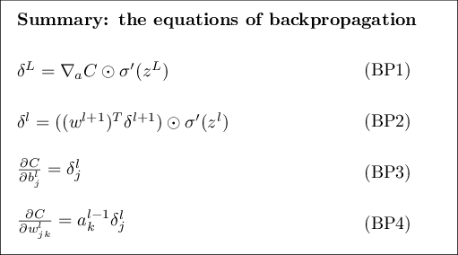
Source: Michael Nielsen
With the four equations in place, I hope it’s clear why it’s called “back”propagation. We first compute the activations forward, and then start at the error of the final layer, then use that to compute the errors of all the previous layers, one by one. With the errors in place, we find out the gradient of the cost with respect to all the weights and biases.
Here’s the logic in pseudocode:
-
Input layer : compute the first activation $a^{1}$
-
Feedforward: compute $z^{l} = w^{l}a^{l-1} + b^{l}$ and $a^{l}=\sigma(z^{l})$ for $l=2,3,…L$
-
Output error: compute $\delta_{j}^{L} = \frac{\partial C}{\partial a_{j}^{L}} \cdot \sigma’(z_{j}^{L})$ at the last layer
-
Backpropagate the error: for each layer $l=L-1, L-2, … 2$ compute $\delta_{j}^{l} = \sum_{k} w_{kj}^{l+1} \delta_{k}^{l+1} \cdot \sigma’(z_{j}^{l})$
-
Gradient: use the error vector for each layer to find $\frac{ \partial C}{\partial b_{j}^{l}}$ and $\frac{ \partial C}{\partial w_{jk}^{l}}$
The actual implementation is:
def backprop(self, x, y):
        zs = [] # Store all the inputs to the neurons
        activations = [x] # Store all the activations, need the input for the first cost gradient wrt weight and bias
        activation = x
        for w,b in zip(self.weights, self.biases): # Feedfoward the input till the final layer
            z = np.dot(w, activation) + b
            zs.append(z)
            activation = sigmoid(z)
            activations.append(activation)
        # Compute the error of the final layer
        delta = self.cost_derivative(activations[-1], y) * sigmoid_prime(zs[-1])
        # Store all the derivatives in the corrrectly shaped matrices
        nabla_b = [np.zeros(b.shape) for b in self.biases]
        nabla_w = [np.zeros(w.shape) for w in self.weights]
        # Backpropagate the erorr to all layers, except the first
        for l in range(2, self.num_layers):
            z = zs[-l]
            sp = sigmoid_prime(z)
            delta = np.dot(self.weights[-l+1].transpose(), delta) * sp # Updates delta at each step, so we don't need to store a list of the errors
            nabla_b[-l] = delta
            nabla_w[-l] = np.dot(delta, activations[-l-1].transpose())
        return (nabla_b, nabla_w)

def cost_derivative(self, final_activation, y): # Partial derivative of the cost with respect to the final activation
        return (final_activation - y)
And just like that we have all the pieces we need for our neural network to classify handwritten digits. Since we take in the 28x28 digit images pixel by pixel, we have 784 neurons in the input layer. The final layer has, as discussed before 10 neurons. The number and size of hidden layers is left to the designer, and I chose to follow Michael Nielsen and have one hidden layer, with 100 neurons.
net = network.Network(sizes=[784, 100, 10])
net.SGD(training_data, epochs=30, mini_batch_size=10, eta=0.001, test_data=test_data)
This modest network achieves ~92% accuracy! State of the art Neural Networks for image tasks, Convolutional Neural Networks have achieved as high as 99% accuracy on this problem.
Resources
It took me ~24 hours (over two weeks) to understand everything that is in this post. While the code is short and seems straightforward, there are many tricky aspects to it, with many crucial subtleties. I would highly recommend proving all 4 equations, then writing all the code yourself to internalize why and how neural networks work.
This is a heavily condensed version of the many things I’ve learnt. The theory and code in the post closely follows the book by Michael Nielsen, an excellent resource with lucid explanations.
Other awesome resources that helped deepen (pun intended) my understanding of neural networks are:
- 3Blue1Brown: the undisputed king of visuals and intuition
- Andrej Karpathy: you will actually enjoy coding and debugging
- Sebastian Lague: a very elaborate and detailed experiment, taught from first principles & explained marvelously
Leave a comment