Charismatic Leadership Tactics Assessment

Predicting leadership qualities using machine learning (and some deep learning) with 77 data points

“He could sell ice to an eskimo”

Why do some people instantly capture attention while others who are just as capable fade into the background? Charisma shapes whose voices rise and whose ideas get heard. Charisma is not the same as intelligence. Some people naturally project confidence, warmth and energy even when their message is simple. Others have great ideas but struggle to communicate them in a way that resonates. These differences shape everyday situations from presentations in class to job interviews and leadership roles. Understanding what makes communication engaging can help train people to become effective communicators.

Charisma includes auditory cues (e.g., tone), linguistic strategies (e.g., anecdotes), and visual signals (e.g., hand gestures). The automated assessment of such traits represents an intersection of Computer Vision, Natural Language Processing, and Psychology. Charisma assessment is inherently challenging because it relies on the integration of heterogeneous cues: no single modality can capture its full complexity. For instance, the perception of “enthusiastic” often emerges from the interplay of an animated tone of voice, specific rhetorical devices, and open body language, rather than any single factor in isolation.

In this post I explain my second group research project @ Maastricht University where we built a system to predict charismatic traits given a video input.

Methodology

Our data comes from a psychological study of university students. The researchers recorded participants speaking impromptu on a given prompt before and after receiving leadership training, and asked people to rate each video across multiple dimensions. These videos are the inputs we use to predict the survey ratings.

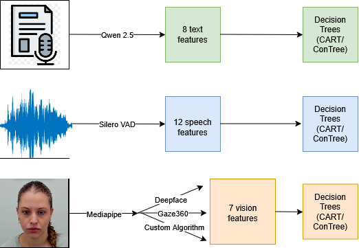
Our final solution involved two stages. First, we extract interpretable features for the three modalities [vision, speech, and text] using different pre-trained deep learning methods. Second, we train Decision Trees on these features to predict the ratings. This division allows for independent development across individual modalities, making combining different results trivial. A visual representation is shown below.

Through our work we hoped to answer four research questions:

• RQ1 Which data modality, by itself, holds the strongest predictive power?
• RQ2 What metrics are relevant for comparing detection across different modalities, and how can they be combined in a meaningful manner?
• RQ3 What multi-modal architectures best balance predictive accuracy and explanatory power for charismatic trait inference from long-form video, audio, and text?
• RQ4 How can agentic frameworks be implemented to provide actionable, intepretable and user specific predictions?

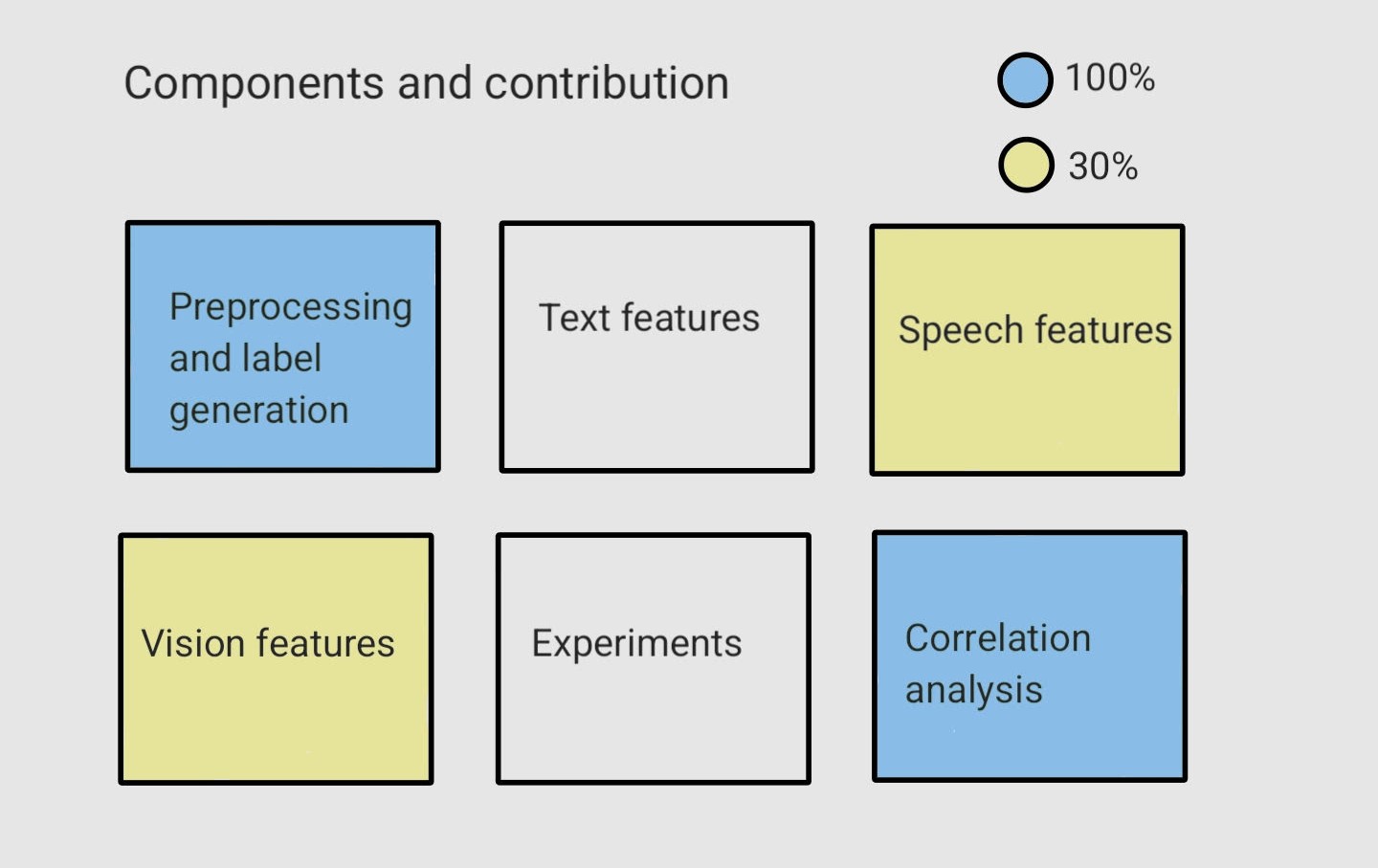
We needed 6 main components to make this all work which are visualized below along with my contribution.

Pre-processing and label generation

I start by explaining the all important labels for the task and how I calculated them for each participant.

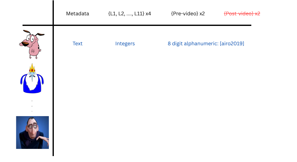
The structure of the survey reviews dataset

Each row here is a single person who rates four different videos, two pre-videos and two post-videos (identified by their unique code). They also enter some meta-data like the type of device they are using and their age and gender. They rate the participants across 17 different charisma dimensions, each score being an integer in a certain range. However, during preprocessing, I found an error in the study, only the pre-videos were shown to the survey respondents. As a result, the usable data contains one video per student, reducing the dataset to 77 unique videos. For this reason we decided not to use deep learning methods directly to make predictions, the models wouldn’t train very well and the high-dimensional embeddings would be undecipherable.

The original survey had 17 labels, to reduce reliance on the most subjective ratings, we excluded five labels. I then cleaned the survey data by (i) removing incomplete responses, (ii) standardizing column names, and (iii) extracting numeric ratings from mixed-format entries (‘1notatall’ $\to$ 1). The label are a mix of multi-modal characteristics (warmth) and uni-modal characteristics (appropriate facial expressions), the full list of the 11 labels is in the Appendix. For each participant, I collect all their ratings from different respondents and finally store their average score per label. Along with these, I also store each participants’ gender (don’t worry we don’t use this to make predictions). All this done, we end up a neat little file with 77 rows and 13 columns.

A few things to note:

• Each video is not shown an equal number of times, and averaging the scores masks this detail. Some videos were clearly more popular than others, any final considerations should take this into account.
• There are almost equal male and females in the study, both in the participants and the respondents themselves. This means there is no need to re-sample the data points for creating a uniform sample.
• Both label ratings and survey responders follow a unimodal distribution without any heavy skews. This means that most students perform similarly well and the critics are not easily impressed or overtly harsh, a good sign. (Plots are in the Appendix)

Vision features

We created 7 interpretable features that rely purely on visual aspects. These are grouped into three main categories: (i) gaze (ii) emotion (iii) body movements. The goal here is to predict a single label that asks if the participant used appropriate facial expressions. I was responsible for catching gaze related events. The full set of features created is in the Appendix.

We processed each video frame by frame and used the Mediapipe detector for extracting facial landmarks. With this in place, we each implemented different models to capture our specific traits.

I used the Gaze360 model to estimate a three-dimensional gaze vector and classified the gaze in each frame into one of two buckets: (a) eye contact (b) looking down. The decision was made by comparing the angle of the gaze vector to the direction of the camera (using some dot products).

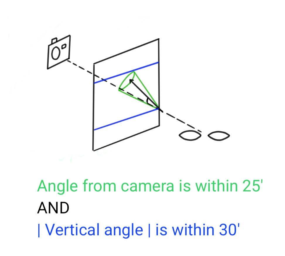
Gaze classification

Essentially if the gaze vector lied in the intersection of the green cone and the blue boundaries, you held eye contact. If the vector’s vertical component ($vsin(\theta)$) fell below the lower threshold you were looking down. Now the problem in this (and the other two methods) is that the constant values for the thresholds come from manually watching the videos and tweaking knobs until the counts matched our own.

For classifying emotions we used the DeepFace model to predict the emotion displayed on each frame. The model detects 7 base emotions which are reduced to either positive or negative emotions. We do this so that we don’t blow up the feature space. On another note, we tried to maintain an equal number of features across modalities. A caveat here is that there were two times negative(angry, disgust, fear, sad) emotions as positive (happy, surprise).

Along with this we also detect smiles. For each frame of the video we generate facial landmarks form Mediapipe. We perform a neat trick to capture only real smiles. A smile is detected only when the person’s lips are spread far apart and their eyes are close together. The thresholds for how far (close) are again set by manual observation.

Finally we counted head-nodding and hand gestures as indicators for body movement. Once again, the facial landmarks are derived from Mediapipe. We used the nose-tip landmark as a proxy for head position and extract its normalized vertical coordinate over time. Nods are then detected by identifying local minima in the trajectory of the landmark over a few frames that exceed a minimum movement amplitude and are sufficiently spaced in time to avoid double-counting.

For each frame we again used Mediapipe to extract landmarks on the hand, and computed a hand-center position by averaging the coordinates and derived a motion signal by calculating the velocity between consecutive hand-center positions. A gesture event is registered when the smoothed velocity exceeds a calibrated threshold.

Speech features

We created 12 interpretable features that rely only on the participant’s speech. The goal here is to predict a single label that asks if the participant used an animated tone of voice. The full set of features created is in the Appendix.

In the videos each person is shown three prompts on a blank screen for 5 seconds each after which they respond. It would be a mistake to classify these segments as speaker pauses. To fix this, we used basic image thresholding to identify the prompt screens and removed them from consideration. Each video is then converted to standardized mono audio to ensure consistent downstream processing.

We then applied the Silero voice activity detection (VAD) model to identify speech segments. These segments are crucial for all the statistical features that we derive from them.

Fluency is characterized using timing-based statistics derived from the structure of speech and silence. We measured overall speaking time, total silence, the number and duration of unusually long pauses, and the longest uninterrupted speech segment. Together, these features captured hesitation, pacing, and the speaker’s ability to sustain continuous speech.

To model vocal expressiveness, we extract pitch statistics from voiced regions only. Pitch variability serves as a proxy for animated versus monotonic delivery, with higher variability generally indicating more expressive speech. In addition, we compute overall vocal energy as a simple measure of loudness and projection.

Text features

We created 8 interpretable features based entirely on the content of the speech, capturing linguistic nuance. These were used to predict 4 labels that can be inferred from this information. As always, the details are in the Appendix.

For each video we generated a reliable transcript using the whisper (medium) model.

These transcripts are then fed into a large language models (LLM) with a consistent, feature-specific template. Each feature is evaluated independently, resulting in one model call per feature per transcript. This design reduces interference between categories and encourages focused, reproducible decisions. All model calls are run deterministically to ensure repeatability.

Apart from the feature counts, each LLM response includes optional supporting evidence drawn directly from the transcript. We applied automatic validation to verify that all quoted evidence appears verbatim in the original text, removing duplicates and invalid entries.

We tested out various models to determine the one most suitable for our dataset. While exact agreement across all features was rare, models showed meaningful differences in per-feature accuracy and error profiles. In particular, more conservative models under-counted, while more aggressive models over-counted. In the end we decided to go with Qwen 2.5 for our LLM counter.

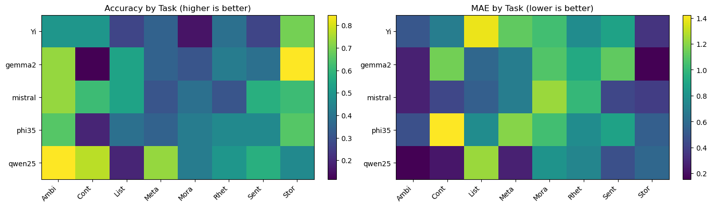
A comparison of the different LLMs tested

A problem unique to the text modality is the sparsity of the feature counts. We suspect that is this is because the items we are looking for are overkill for the speakers in question. A vast majority of them don’t use complex lexical tools and convey their ideas in simple language. I visualize below just how dire the situation is

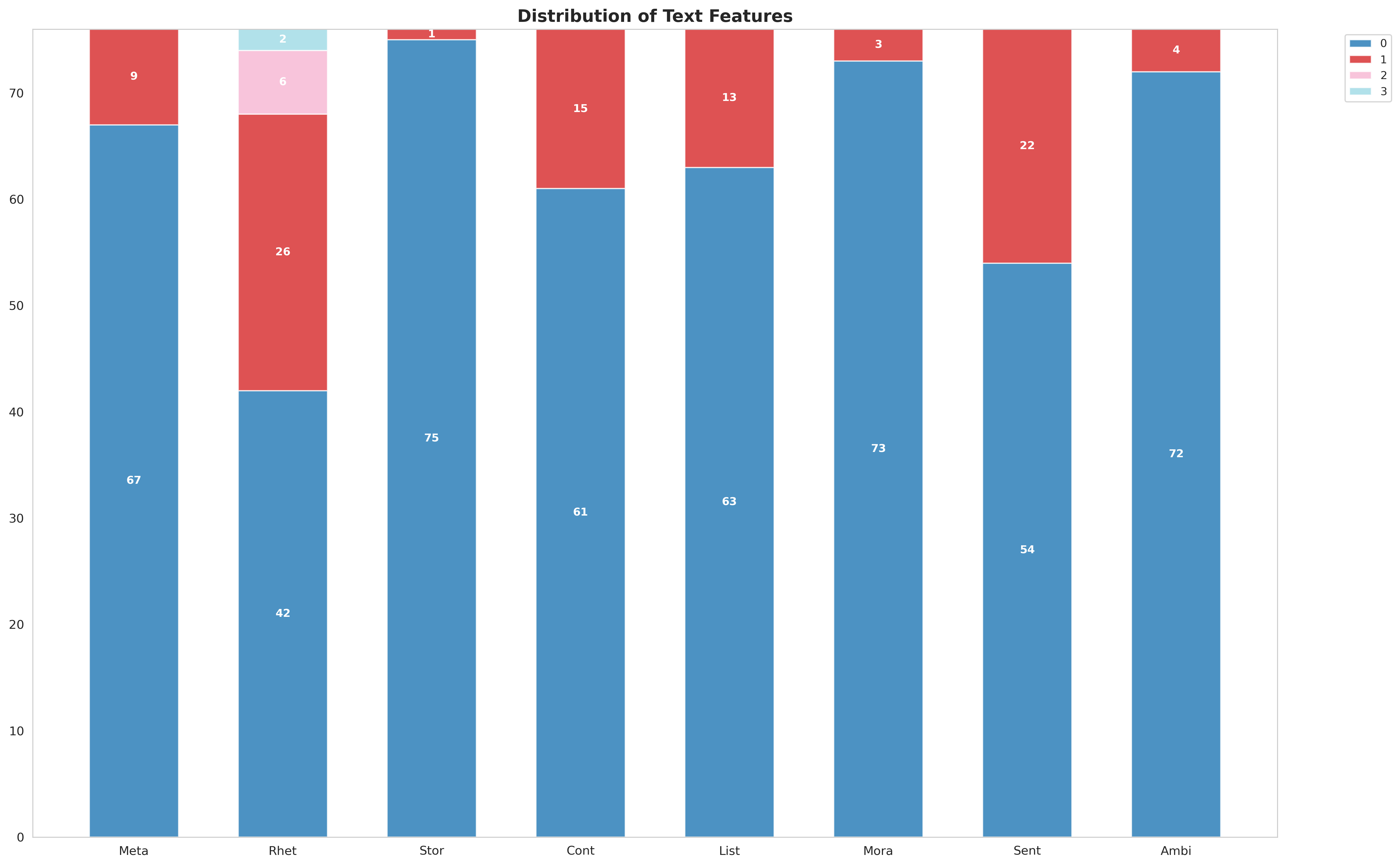
Most text features are 0!

Experiments and results

Phew, that was a lot of words. Before we move on to the experimental set up and the findings, here’s a quick overview of the three features and some interesting properties.

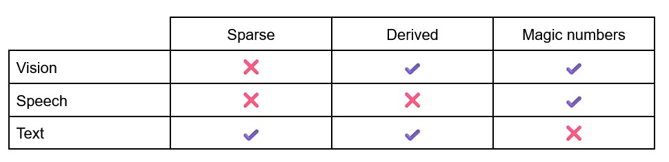
The vision features reply heavily on manual thresholds (gaze, body motion, emotion) informed by three people watching a limited number of different videos. Luckily most counts are non-zero, which means the decision trees can work reliably.

The features drawn from speech are purely statistical, they do little to almost no post processing and are as close to the raw input signal as possible. Luckily, they don’t suffer from as much sparsity as the text modality. Unfortunately the minimum duration of pauses (5 sec) is set manually based on limited videos. This one issue stops it from being the almost ideal set of features!

Text on the other hand is hit hard by sparsity, which is probably the major reason for it’s poor performance. It should be noted that the features prescribed to us were maybe overkill given that the participants in question were amateurs in training and not seasoned orators. It is still a derived feature, although this is not a concern given the meteoric rise in LLMs’ language processing. This was the one set of features that was free of any manual thresholds, and while it still relies on labels, no manual tweaks are needed, making it that much better.

Decision trees

We wanted a uniform a consistent set-up to evaluate and compare performance across the modalities. We used the Leave-One-Out Cross-Validation (LOOCV) error for gauging model performance. We fit ConTree and CART flavors of Decision Trees in each case. We predicted the average value of the label in question for baseline performance.

Uni-modal

In the case of vision and speech, there was only a single label to predict. This made the experimental setup very easy. For the speech modality CART trees of depth 2 (super shallow) beat the baseline by ~15%. On the vision modality, CART trees of depth 3 (still super shallow) were able to beat the baseline by ~26%.

Since we had to predict 4 labels from 8 features for the text modality, we had two experiments to run. Predicting each label one using a single feature and predicting all labels with all features. Sadly both of these performed very close to the baseline.

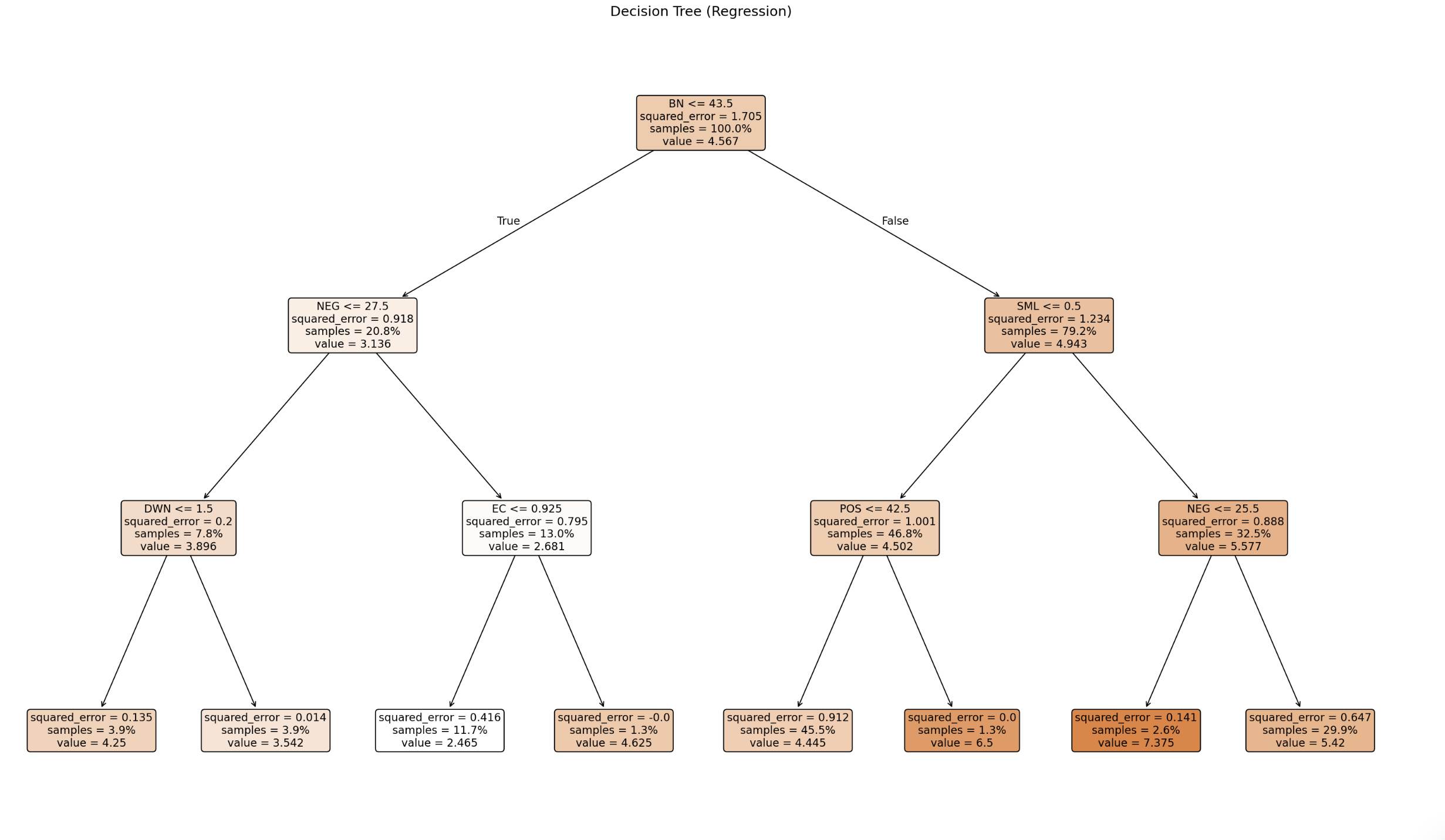
Here’s an example decision tree, from the speech modality

The main results aside we performed a quick sanity check to see if an LLM predicting the text labels from transcripts could lead to better result than our long-winded approach. Luckily for us it performed much worse, and paradoxically made us feel better about our not so great text features. It should be noted that this was a case of zero-shot learning since the LLM had no prior labeled examples to work with.

Multi-modal

We had 5 multi-modal labels to predict and 28 uni-modal features across three modalities. Again there were two results to compare: predicting multi-modal labels with modality specific features and predicting multi-modal labels with all features together.

In the uni-modal feature settings, speech was by far the best at predicting all 5 multi-modal labels. Interestingly the text features beat the vision features on all the 5 multi-modal labels!

Using all features together beat the baseline for labels L1, L2 and L4. The best performer was a ConTree of depth 2 which utilized vision and speech features but did not pick text features at all. There seems to be some interesting, non-intuitive relationship among labels and features that needs to be understood and explained.

Correlation analysis

There is a lot going on here, in labels and features. We conducted three sets of visualizations to examine the distribution of the charisma scores and to identify potential clusters indicative of underlying traits. Given the limited sample size, we avoided applying clustering algorithms, as these would likely produce spurious or unreliable associations.

The following relationships were analyzed:

1. Uni-modal labels versus Uni-modal features

2. Multi-modal labels versus Uni-modal features

3. Multi-modal labels versus Uni-modal labels

No meaningful relationships were observed for cases 1 and 2. Interestingly, this absence of results proved an interesting result in the speech modality. In the plot below male participants are colored blue while their female counterparts are colored pink.

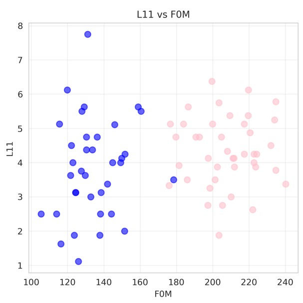
Animated tone of voice as a function of pitch

A clear separation between male and female participants is evident. Despite the pronounced difference in pitch between genders, there is no apparent systematic bias in the associated speech labels, as both male and female participants exhibit similar label values. This observation speaks to the un-biased ness of the survey respondents.

I missed a rather crucial observation by analyzing case 3 at the very end. The labels in our case come from self reported surveys, and are in no way required to be independent of each other. Below is a plot revealing just how closely most of the labels are in this case.

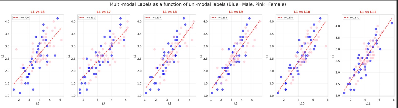
“Charismatic” compared to the other labels

The minimum Pearson correlation coefficient observed in this case is 0.726, with an average correlation of approximately 0.75 in total! This strong correlation may stem from the structure of the survey itself, including the order in which questions were presented and the amount of time respondents devoted to each question. These effects arise solely from the the collected data and are independent of the features extracted in our analysis. It’s unlikely that I give a person a low score on facial expressions if I find them enthusiastic ..

This result suggests that modeling can focus predicting the easiest sub-modality using explainable features, with the results subsequently used to infer multi-modal labels. This simplifies the approach while maintaining strong performance.

What’s next?

I like to think our work mainly informs the next group what not to do! I quit joking around and articulate directions of future work below:

• Reliable ground truths for features: we came up with the explainable features ourselves, checking each model’s performance against manual performance on the same input. For quality feature generation I would start by finding some reliable and repeatable means of ground truth, enhancing the quality of features and hopefully the final predictions too.

• Reduce or remove magic numbers: all three systems in vision and the logic in speech relied on thresholds estimated by various members of the team on independent videos. Apart from this systemic problem, this solution does not scale and is heavily biased on the samples selected. A deeper analysis of the data can be performed to guide machine learning approaches apart from any insights from literature.

• Multi-dimensional correlation: the correlation done in this instance was binary, only a pair of (label (or) feature) were compared. We know from psychology that Charisma is a multi-modal phenomena, so visualizing the ‘Warmth’ label as a linear combination of uni-modal features might be a good starting point. A more thorough study of this topic is sure to produce non-trivial insights. Care must be made that the combinations scale exponentially and the signal to noise ratio is extremely small.

• Temporal features: we had hoped to build a temporal database of features across each modality. This could then be fed into an LLM for mildly sophisticated reasoning. One could then expect responses like ‘Your rating for confidence is low, you seem to smile only near the end unlike your peers with high scores who smile at [x,y,z].’ A basic setup was created by storing the frames that lead to a certain decision but was not fully developed and integrated. Creating a data representation with temporal aspects can lead not only to higher predictability but also interpretability.

• Feature engineering: although it was easy to spo that we needed new features on the text modality sue to their sparsity, non-zero counts are not a seal of quality. The next team needs to critically evaluate the set of features we’ve proposed across all modalities and come up with something more suitable for the dataset in question while being grounded in literature / practice.

Appendix

Below you will find a long list of all the labels and their meanings, along with all the plots did not fit in the main post.

Labels:

Multi-modal

• L1: Charismatic
• L2: Likable
• L3: Warm
• L4: Enthusiastic
• L5: Inspiring

Text

• L6: Has a clear understanding of where we are going
• L7: Paints an interesting picture of where we are going as a group
• L8: Inspires others with his/her plans for the future
• L9: Able to get others committed to his/her dream

Vision

• L10: Uses appropriate facial expressions

Speech

• L11: Uses an animated tone of voice

Features:

Text

• Meta: Uses a metaphor (count)
• Rhet: Poses a rhetorical question (count)
• Stor: Tells a story or anecdote (count)
• Cont: Uses a contrast (count)
• List: Uses a list (with 3 or more parts) (count)
• Mora: Makes a moral appeal (count)
• Sent: Expresses the sentiment of the collective (count)
• Ambi: Sets an ambitious goal (count)

Vision

• HM: Hand movements (count, number of frames)
• BN: Body sway (count, number of frames)
• DWN: Looking down (count, number of frames)
• EC: Eye contact (float, percentage of eye contact was held)
• POS: Positive emotions (count, number of frames)
• NEG: Negative emotions (count, number of frames)
• SML: Smiles (count, number of frames)

Speech

• DUR: Duration (seconds, entire video length)
• ST: Speech time (seconds, talking length)
• SILT: Silence time (seconds, silence length)
• NP: Number of pauses (count)
• MP: Mean duration of pauses (seconds)
• MXP: Maximum pause duration (seconds)
• MXS: Maximum speech duration (seconds)
• F0M: F0 Mean
• F0STD: F0 Standard deviation
• F0R: F0 Range
• RMSE: RMS Energy
• FC: Filler count (count)

Graphs

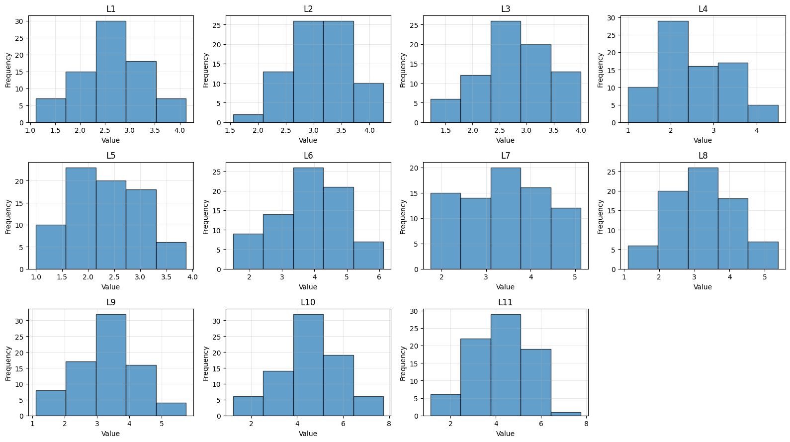
Distribution of participant scores

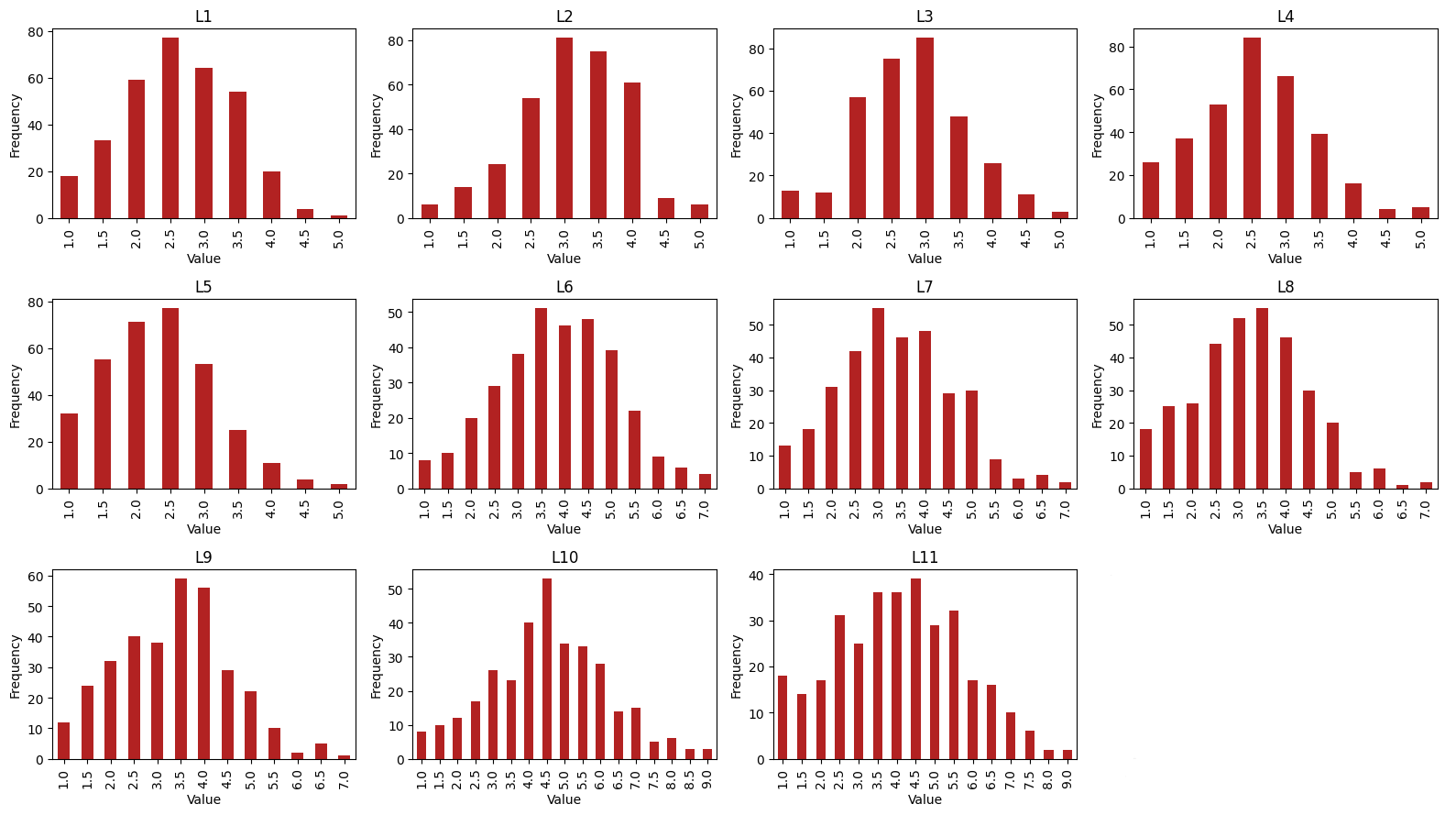
Distribution of survey responders ratings habits

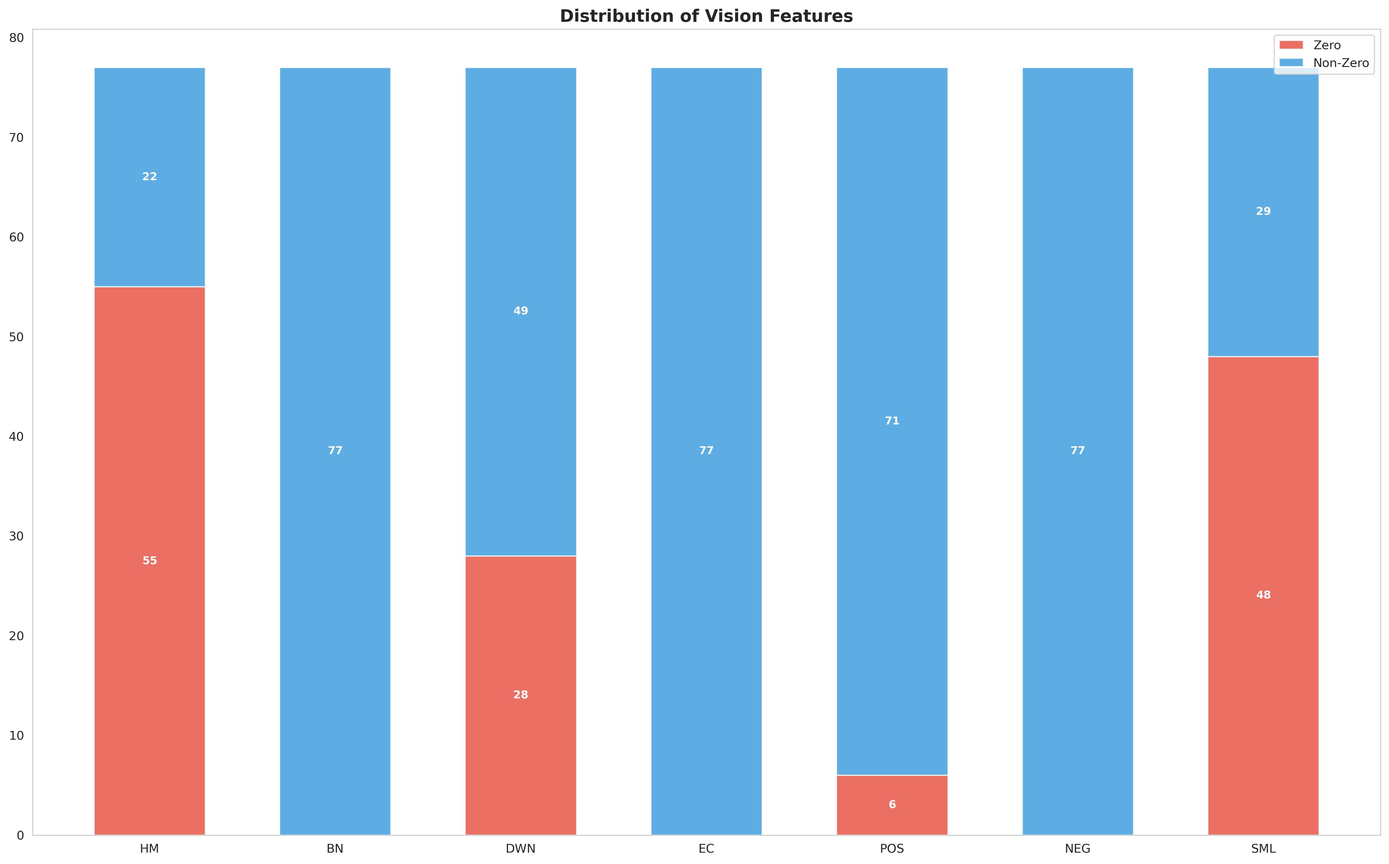
Distribution of vision features

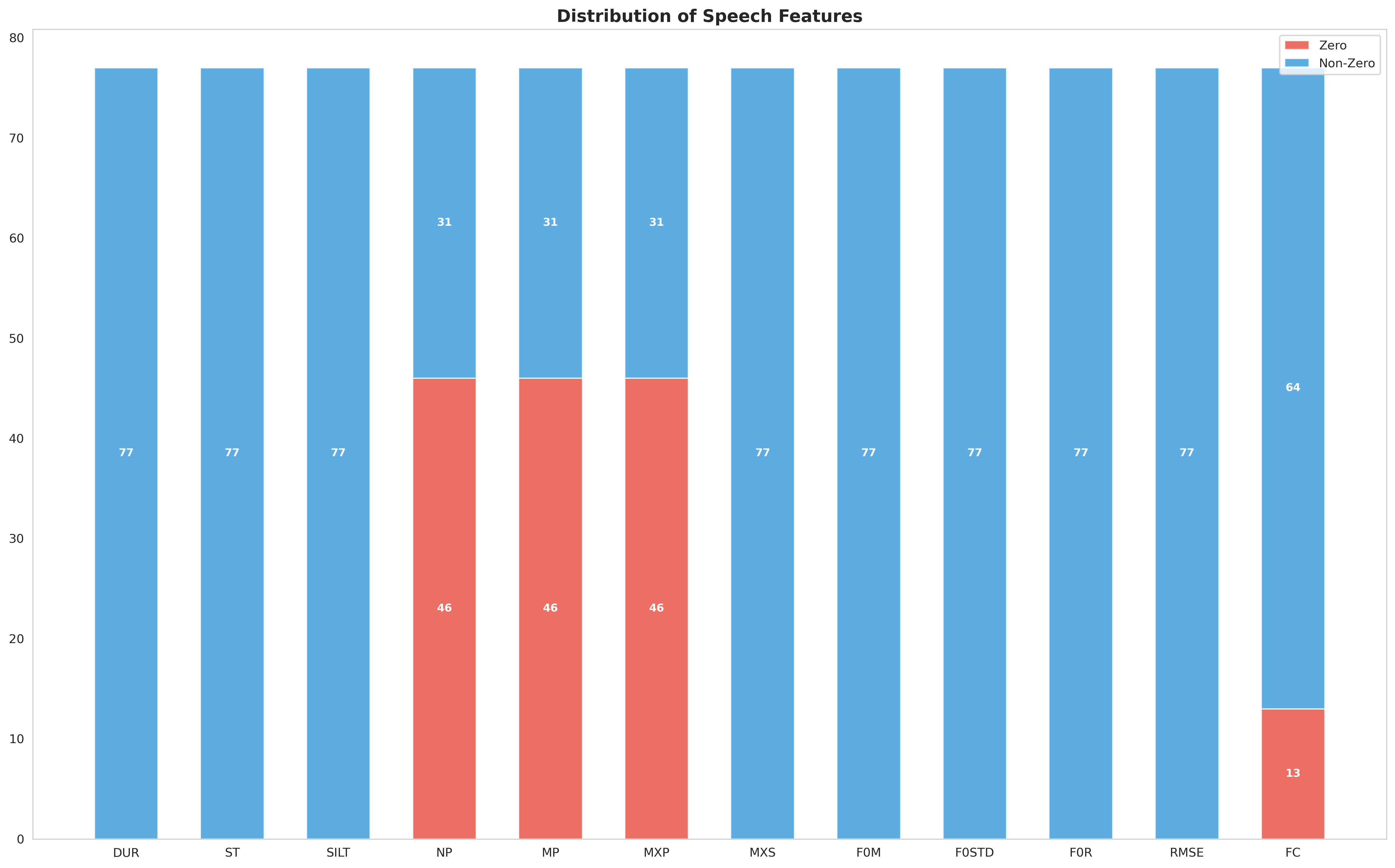
Distribution of speech features