Chapter 8: Tree-based Methods

From linear regression to smoothing splines, all the algorithms we have studied so far make some assumption about the functional relationship between the predictors and response. In this chapter we learn an algorithm that doesn’t make any assumptions whatsoever about f!

It’s going to really feel like a computer science algorithm 😔 Luckily the output that decision trees produce can be understood by humans just fine, and that’s where we will start, with an example.

Regression trees

Let’s try to build a tree that predicts the salaries of baseball players (in thousands of dollars) based on the number of years they have played for & the hits they made in the last season.

A regression decision tree. (Source : ISL Python)

We can interpret a decision tree as a cascading set of if-else conditions. In the example above, if a player has played for less than 4.5 years they are predicted to earn 5,000$. On the other hand, if they have played for longer than 4.5 years and made more than 117.5 hits, they earn 6,740$.

How exactly did we arrive at the numbers 4.5 & 117.5? How did we know to pick years and hits? In order to understand that, we need to see another view of decision trees. Each decision or condition in a tree, splits the data points into smaller sub regions. It’s these sub regions that the algorithm optimizes over.

The 3 sub regions created by the decision tree. (Source : ISL Python)

The number of sub regions depends on the number of conditions ( decision nodes) we want our tree to have. More decision nodes will lead to more sub regions. The tree takes an average of all the points in a given region and predicts that singular number as the output for any other point that ends up in the same box. That is all players that fall in R1 are predicted to have a salary of 5,000$.

Decision trees is a brute force algorithm. At each decision node it considers all possible predictors (X_j) and the values that they can take (s), so that the resulting sub splits (R1, R2) have the lowest combined RSS. This is equivalent to finding j and s that minimizes

It performs this brute force optimization at each step. We notice that one predictor can be picked more than once, albeit with a different threshold value. The total number of splits and minimum number of data points in each split are defined by the user.

Classification trees

We can also use decision trees for classification tasks. However we cannot use RSS as the metric to run our optimization algorithm on, since responses are qualitative and not quantitative.

Another difference this leads to is that the predictions that are made are based on the majority class in a given region. Let us assume that one region has the following observations {red, red, green} then all the observations that land in that region are predicted as belonging to the red class.

We need metrics that measure how pure a set of observations are. A measure of the ratio of classes present in any given region. Two popular metrics to do this are the Gini index and entropy, defined as below

Both of these measure the total variance across K classes and have similar values numerically ; notice they both are small when p_mk is 0/1. Since they measure variance and we are interested in a region’s purity, these quantities need to be minimized across both split regions.

Classification decision tree. (Source : ISL Python)

In the above example we see a classification tree predicting whether or not a person has heart disease based on predictors like heart rate, chest pain, etc.

Notice something curious here, there are 2 places where the splits lead to two No and two Yes predictions! This is not an error, remember that the predictions made are based on the majority class of a region. The split has resulted in higher purity, which means that both regions have a majority of the No/Yes class. This only improves prediction accuracy.

The optimal depth of the tree (number of decision nodes) & minimum samples for a given problem is found by cross validation.

Advantages and disadvantages of trees

But why go through all this trouble? Why not just do linear regression? There is no one algorithm that fits all models. If the true relationship b/w predictors and response is linear, linear regression will trump decision trees. But in the case of more complex, non-linear relationships we expect decision trees to perform better.

Binary classification. (Source : ISL Python)

In the above example we see a simple example with two classes, illustrating the different scenarios discussed above.

Decision trees have many advantages :

• Interpretable ; easier to explain than linear regression, especially for non-technical stakeholders
• Graphical interpretation is always possible, regardless of dimensionality
• Can easily handle qualitative variables without creating dummy variables

But they are also lacking in some ways

• Low prediction accuracy due to averaging / majority
• High variance, a small change in the data can cause a change in the final tree

In order to mitigate the cons of decision trees, we will use ensemble methods. Ensemble methods are an approach that combine many “building block” models in order to make one single (and potentially powerful) model.

Bagging

We know that averaging over many samples leads to a reduction in the variance. So the best case scenario would be to train a decision tree over multiple training sets and average the predictions. Hold up… we don’t have so many training observations. So we do the next best thing, bootstrap (from chapter 5.

In bagging we take repeated (random with replacement) samples from a single data set in order to make B bootstrapped training sets. We then fit B decision trees and then average the predictions.

Once we do this for all data points x in the original training set, we have our bagging decision tree. Each individual tree has high variance and low bias, but by combining individual trees we have a resultant tree with low variance and high bias. Bagging works well by combining hundreds and thousands of trees into one single procedure.

A visual representation of Bagging. (Source : AIML)

If the number of trees B is very large, we run the risk of over-fitting. Another thing to notice is that the data sets used in bagging are highly correlated.

Random forests

Random forests again produce B bootstrapped training data sets. At each decision node we pick the best predictor out of m < p predictors picked at random. At each step the predictors in consideration are drawn randomly.

Effectively while building the random forest the algorithm is not even allowed to consider a majority of the predictors. The rationale behind this is that if there is one predictor highly correlated with the response, then all the trees in bagging will pick that to be the first predictor. Consequently all the trees will look similar. With random forests (p-m)/p tress won’t even consider that predictor, giving other predictors a higher chance.

This means that although the training data sets are correlated, each decision tree is now decorrelated, since it uses a different set of predictors. When m=p it is the same as bagging.

Variation in test error of random forests. (Source : ISL Python)

In the above graphic we see the variation in test error in random forests as a function of the number of trees & number of predictors. We see that sqrt(p) works better than p in this case. In general a small value of p works well when we have a large number of correlated variables. One use case of random forests is gene expression data, which is high dimensional.

Boosting

Unlike bagging and random forests, boosting works on a modified version of the original data. I will list out the algorithm and then explain how it works and why this is a good approach

The boosting algorithm. (Source : ISL Python)

Instead of fitting a single large decision tree to the data, the boosting approach learns slowly. The idea is to build a model that learns successively from the previous trees.

We start with our final model set to 0, with the residuals being the observations. We then build B-1 trees on the training data. At each step i we update the final model by adding a shrunken value of the i^th tree. We also update the residuals by adding a shrunken value of the predictions. The final decision tree is thus a sum of all these shrunken decision trees.

Visualizing boosting decision trees. (Source : ResearchGate)

Hence we fit the decision trees to the residuals instead of the response Y. By fitting the trees on the residuals we slowly improve f in areas it doesn’t perform well. The shrinkage parameter λ slows the process down even further, allowing more and different shaped trees to form.

There are 3 parameters we can tune in the boosting algorithm :

• Number of trees (B) : boosting can overfit if the number of trees is very large, the optimal number of trees is found using cross validation.
• Shrinkage parameter (λ) : controls the learning rate, usually 0.01/0.001. Very small λ can require a very large B to be effective.
• Number of splits (d) : controls the depth & complexity of the tree. Usually d=1, a tree with a single split (stump) works well.

Boosting v/s Random Forests. (Source : ISL Python)

In the above graph we see a comparison between boosting and random forests for gene expression data. We see that even stumps (d=1,2) can outperform random forests if enough trees are considered.

This highlights one difference between random forests and boosting ; because the growth of a particular tree takes into account the trees that have been grown, smaller trees are typically sufficient.

Bayesian Additive Regression Trees (BART)

In bagging and random forests we made bootstrapped data sets and built independent trees, the final model was then an average of these trees. In boosting we used a weighted sum of trees, fitting onto the residual. Each new tree tries to capture a signal that was missing before.

BART is like an intersection of the two methods. Each tree is constructed in a random manner and it tries to capture a signal not accounted for. Let K denote the number of decision trees and B denote the number of times we run the BART algorithm.

At the end of each iteration, the K trees from from that iteration will be summed to form the final prediction at that level. In the first iteration all the trees are initialized such that their sum is the mean of the observations.

In subsequent iterations BART updates the K trees one at a time. In the bth iteration, to update the kth tree, we subtract from each response value the predictions from all but the kth tree. This results in a partial residual.

Instead of fitting a new tree on this residual, BART randomly chooses a perturbation from the tree of the previous iteration i.e. f_k @ iteration b-1. Here a perturbation is (i) adding / pruning a branch (decision node) (ii) changing the prediction of a given node. We try to improve the fit of the current partial residual by modifying the tree obtained in the previous iteration.

Once this process is done for all K trees, we find the sum which forms the prediction for the bth iteration.

We typically throw away the first few iterations since they don’t return good results. This is called a burn in period.

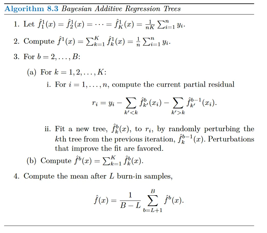The BART algorithm. (Source : ISL Python)

Since we slightly improve the tree from the previous iteration as opposed to fitting a fresh tree, this limits the tree size, preventing over-fitting.

BART v/s Boosting. (Source : ISL Python)

In the above graphic we see training and testing errors for two algorithms as a function of number of iterations. The grey area represents the burn in period. We notice that the BART test error remains constant as the number of iterations increases, whereas the boosting test error increases at large iterations, over-fitting on the training data. I will end this discussion with an easy to understand visualization of the BART algorithm.

BART but easy to understand. (Source : ISL Python)

Here is a summary of the ensemble methods discussed

I apologize that this post took so long. I have been caught up with some grunt work the last few weeks. I hope to stick to schedule and finish the remaining chapters on time :’)