Chapter 7: Moving Beyond Linearity

A pool shaped like a sine wave ; non-linearity! (Source : Unsplash)

While linear regression / classification is a good place to start any analysis, it is rarely the case that the true relationship is linear. And so after 6 long chapters, we finally start work on non-linear algorithms.

In this post we will explore some parametric (assuming the functional form f) methods to directly extend the linear regression model. For this analysis, we consider a simple example. Trying to predict wage(in thousands of dollars) based on age & education.

We expect wage to increase linearly with education, but with age it increases until a point (40’s–50’s) and then starts to reduce. Intuitively we expect this to be a parabola, some second order polynomial. Let’s see how this plays out.

Polynomial regression

The most straightforward way to extend the linear model is to include higher powers of the predictors (x) to predict the response (y).

The problem is now reduced to standard linear regression on predictors x, x², x³ … Theoretically the power d in the above equation can be any number, but in general you restrict yourself to 3–4 in order to prevent over-fitting.

We can adopt this same approach for classification tasks as well. Instead of raising the exponential function to linear functions of x, we now raise them to quadratic functions of x. This results in a quadratic log odds.

Fitting a degree 4 polynomial to predict wage using age returns the following results.

Polynomial regression and classification. (Source : ISL Python)

In the above plot the solid lines represent the polynomial function and the dashed lines represent the 95% confidence intervals. We notice two things here : (1) predicting high salaried individuals is hard (>250,000) (2) the standard deviations increase with age.

Step functions

Here we take a more local approach to linear regression. Instead of fitting one straight line on all the data points, we divide the data points into k sub parts and fit a different straight line on each sub part (piecewise linear). These sub parts are called bins.

We do this using indicator functions. An indicator function takes on a value of 1 when a condition is met and is 0 otherwise. In this case we want to check if a given point lies in one of k bins.

In our example this would be checking if a certain age (21) belongs to a certain age bin (20–25). We create k such indicator functions to cover all the data points, and use them as our predictors. This takes the following functional form :

Here we notice that atmost one of these coefficients(excluding the constant) can be 1, since any one point can belong to only one bin. Another thing is that all the indicator functions must sum to 1 ; the point has got to be somewhere! Let’s now try to understand what the coefficients represent.

Therefore the coefficients each represent the average increase in the response (y) relative to the intercept (β_0), this nature gives a “step” nature to the function, with y increasing / decreasing across each bin.

A step function with 3 indicator functions. (Source : ISL Python)

Regression splines

This is just a slight modification of the previous idea, wherein we apply polynomial functions to the k bins ; piecewise polynomials. The points we chose to make the bins in this case are called knots. I will formulate the regression spline equation for one knot, leaving the detailed exposition in the textbook.

However, it isn’t as simple as it looks. In order for us to have a smooth function across knots we need to impose some conditions. Let’s see what this looks like in practice.

Different regression splines. (Source : ISL Python)

An unconstrained regression spline (blue) breaks off at the knot. Imposing the function to be continuous at the knot leaves it with a small hump (green). If the function and it’s first & second derivatives are continuous at the knot, we obtain a smooth (orange) spline.

A natural spline is a regression spline with additional boundary constraints, the function is required to be linear in the boundaries (first and last bins). This helps in reduce the variability (confidence intervals) in the end points.

Natural spline v/s regression spline. (Source : ISL Python)

We now have 2 questions to consider : (1) how many knots do we use? (2) where do we place said knots?

We find the optimal # of knots through cross-validation, taking different # of knots and evaluating their resulting mean squared errors. While it makes sense to have more knots regions with higher variance and fewer knots in regions with lower variation, in practice we place the knots equally through the data.

Smoothing splines

The goal of linear regression is to find a function g(x) that minimizes the residual sum of squares (RSS). Now the lowest RSS is 0 which can be achieved by fitting the line to each and every point. But that would leave the model overly flexible. We need some way to make the curve smooth.

Smoothing splines do this by minimizing the variability in the function, by limiting the rate of change of the function (something that is captured in the first derivative). This leads to the following optimization problem

It turns out that this problem is solved by a natural spline with n knots (where n is the total # of data points)!

At λ=0 our model is highly flexible (high variance). As λ increases, the function becomes more smoother (increasing bias). When λ=∞ we end up with simple linear regression.

Similar to finding the optimal # of knots, the best λ is found by cross validation.

Smoothing splines with different λ. (Source : ISL Python)

In the above plot the splines are plotted as a function of the degrees of freedom which are inversely proportional to λ. Hence higher degrees of freedom lead to a more wiggly (flexible) fit.

Local regression

Remember k-nearest neighbors? This method is quite similar to that. It estimates the least squares line around some test point x_0 using it’s k nearest neighbors. Hence the name local regression. I will outline the algorithm below.

1. Gather the k points closest to the test point x_0   
  
2. Assign a weight k_i0 to each point in the neighborhood such that furthest  
   point has weight 0 and closest has weight 1  
  
3. Fit a weighted least sqaures that minimizes   
   Σ k_i0(y_i - β_0 - β_1 x_i)^2  
  
4. The resulting coefficient estimates form the least squares line

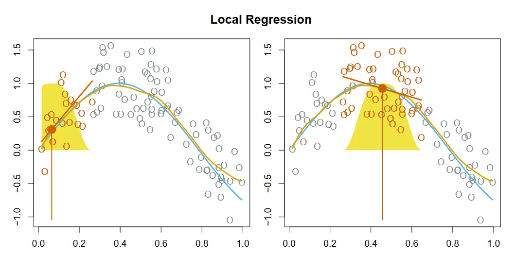Local regression at 2 points. (Source : ISL Python)

In the above graphic the filled red point is the test point x_0, while the hollow red points represent the k nearest neighbors. The yellow Gaussian function indicates the distance of the points from the test point.

Generative Additive Models (GAM)

This is the non-linear extension to multiple linear regression. Here we assign a different transformation to each predictor, depending on it’s contribution. The model is additive since we add individually transformed predictors to model the response.

Consider predicting wage using the calendar year, age and education. In this case education is a categorical variable with 6 levels. We will fit a GAM model to this, using natural splines for the calendar year & age. For education the function uses dummy variable linear regression.

GAM used to predict wage from year, age & education. (Source : ISL Python)

This approach can similarly be applied for classification, with the log odds now being a sum of different functions.

One important benefit of GAMs is that they can help examine the individual effect of each predictor x_j separately. They are however restricted to be additive, missing any relations in the predictors. But this can be easily solved using interaction effects.

Phew, that was a lot. Here’s a quick summary of all 6 methods

In this chapter we could rely on intuition, but in the next chapter we will not be able to. We will learn about our second non-parametric method (after k-nearest neighbors), decision trees.

Spoiler alert : I’ve already worked with decision trees before this and written a blog post too (one of my most popular).