Chapter 6: Linear Model Selection & Regularisation

So far we have only considered cases when the number of observations is much more than the number of predictors, i.e. n»p. And it was a good place to get started, but with big data comes big dimensions. We are now capable of measuring an astoundingly large number of variables.

DNA can contain gene expression levels for thousands of genes! But due to prohibitive costs (among other reasons), we can only have a few observations at hand. Imagine trying to fit linear regression with p=2,000 and n=100 in order to predict the chance of a disease.

In this post I will explain 3 ways of dealing with high dimensional data : (i) subset selection (ii) shrinkage methods (iii) dimension reduction. I will be considering the linear regression algorithm for each of the cases presented below.

But wait a minute… why can’t we just use all the predictors? Short answer, even biased models like linear regression overfit the data.

Now the explanation (even though you didn’t ask). High dimensional data is often sparse, the most popular example being Netflix movie reviews. Sparse data has many values that are missing, in our gene expression example each patient tested will have most genes showing little to no activity (expression). This means that the p columns will be filled with 0’s with a few 1’s sprinkled in.

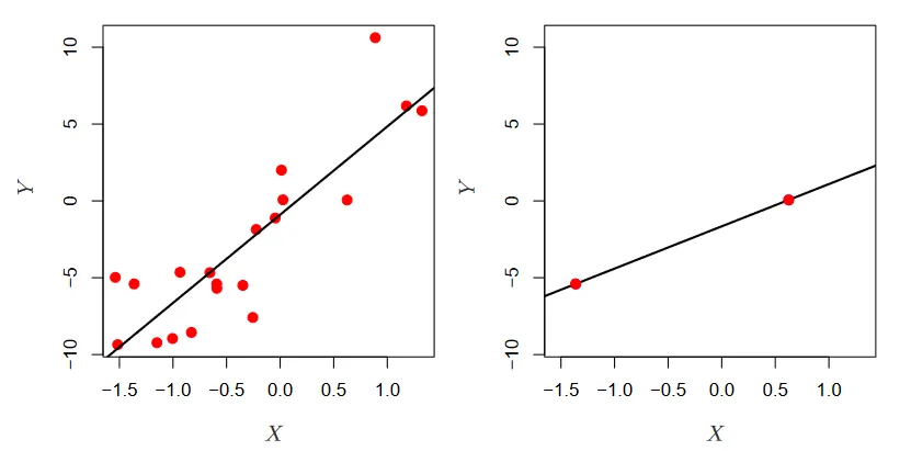The problem with high dimensional data. (Source : ISL Python)

In the picture above we see low dimensional data on the left, and high dimensional data on the right. Linear regression works well when there are lots of observations, minimizing the residual sum of squares. However, with only 2 observations there is only line we can draw, which is in most cases overfitting → drawing incorrect inferences.

Thus we see that the curse of dimensionality haunts even the simple linearity assumption.

With some clarity on why we should change / modify our approach with high dimensional data, we forage ahead.

Note 🚨 : While these metrics are important, they only give us an estimate of training error (the one that doesn’t matter). Take care to use cross-validation and other methods to estimate the test error before zeroing in on a model.

Subset selection

In this approach, we take m < p predictors to train our model on.

The question we need to answer then is, how do we know which m predictors to pick?

(a) Best subset selection (Brute Force)

Fit an individual model on each possible combination using k (k=0,1,…,p) predictors. Then find the best model for each number of predictors. So we fit all models with 1 predictor, 2 predictors … and so on. Then we find the best model at each level, and pick that.

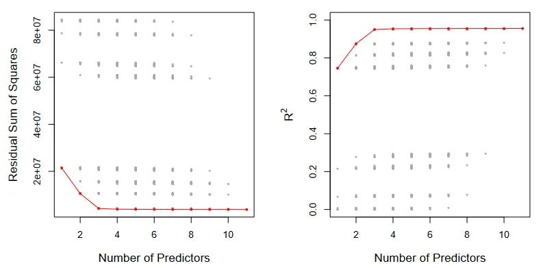Best subset selection. (Source : ISL Python)

In the above picture, all the possible models are shown in gray while the most optimal models are connected in red. As expected, the RSS decreases monotonically and the R² increases monotonically.

By definition, this will give us the best model we can pick. But practically it has some drawbacks. There are a total of 2^p possible subsets making it computationally expensive & infeasible (p=40 yields 10¹³ combination imagine p=2,000) to fit a model on each combination. In order to deal with this we devise two algorithms to help reduce the computational cost.

(b) Forward stepwise

1. Let M_0 denote the null model, which contains no predictors.  
  
2. For k = 0, . . . , p − 1:  
  
  (a) Consider all p − k models that augment the predictors in M_k  
      with one additional predictor.  
  (b) Choose the best among these p − k models, and call it M_k+1.  
      Here best is defined as having smallest RSS or highest R^2.  
  
3. Select a single best model from among M_0 , . . . , M_p using the pre-  
diction error on a validation set, C_p (AIC), BIC, or adjusted R^2. Or  
use the cross-validation method.

(c) Backward stepwise

1. Let M_p denote the full model, which contains all p predictors.  
  
2. For k = p, p − 1, . . . , 1:  
  
  (a) Consider all k models that contain all but one of the predictors  
      in M k , for a total of k − 1 predictors.  
  (b) Choose the best among these k models, and call it M k−1. Here  
      best is defined as having smallest RSS or highest R 2.  
  
3. Select a single best model from among M_0 , . . . , M_p using the pre-  
diction error on a validation set, C_p (AIC), BIC, or adjusted R^2. Or  
use the cross-validation method.

The models in (b) and (c) have running times of ~ p² a major improvement over 2^p of best subset selection.

We notice that both these methods only include the next best or exclude the next worst model. This means that the model with k predictors is a subset of the model with k+1 predictors.

This subset property comes at a cost. The k predictors that worked best need not always be the best at the k+1 level, leading to a hit in accuracy. This effect can possibly compound as we traverse through the entire predictor space.

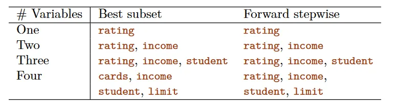Diverging predictors. (Source : ISL Python)

In the example above we see that until 3 variables, forward stepwise selection is finding the best solution. But with 4 variables, forward stepwise picks variables that give sub optimal values. This means that the errors in models picked out by (b) and (c) will always be greater than the one picked out by best subset selection.

There are also other methods that combine the models in (b) and (c) but those are out of the scope of this post.

Shrinkage methods

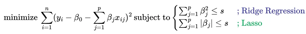
In similar vein to subset selection, shrinkage methods aim to nudge the predictor coefficients (β_j) in linear regression towards 0. It does this by adding an optimization condition (penalty) to the linear regression model directly. Two shrinkage methods are formulated below

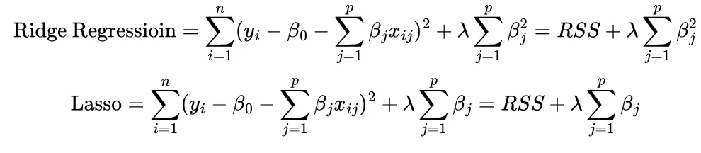
Ridge regression tries to reduce the squared sum of coefficient estimates (β²) while lasso tries to reduce the sum of the coefficient estimates (β). λ is called the tuning parameter ; when λ=0 we revert to the original least squares model and when λ= ∞ we have a model with no predictors. Finding a balance with λ therefore helps us identify which predictors to remove (or reduce in magnitude).

Visualizing shrinkage methods. (Source : ISL Python)

In the above plot we see the coefficient estimates of a data set involving credit card data vary as a function of λ. The left hand panel depicts ridge regression while the right depicts the lasso. We observe that the coefficients start out with large magnitudes (when λ=0) and their net magnitudes decrease monotonically (as λ increases) towards 0.

One difference in these methods is that the lasso can yield coefficient estimates exactly equal to 0, and hence can perform subset selection. Ridge regression however, cannot provide exact zero estimates.

Written this way, we can plot 2 separate spaces, with the full solution lying in the intersection of both spaces. Let’s visualize this for a 2 dimensional example.

The solution spaces. (Source : ISL Python)

In the above graphic the RSS estimates are shown in orange ellipses (with the minimum being the black dot) and the constraint region is shown in blue. The full solution is the intersection of the two spaces. The left hand panel depicts lasso, while the right depicts ridge regression.

Here we see that that the lasso solution lies on the β_2 axis, therefore setting β_1=0. In the case of ridge regression, the intersection does not lie on either axis, thereby not yielding exact 0 but close to 0 values for the coefficient estimates.

To understand this difference we need to differentiate the ridge regression and lasso equations with respect to β and set them to 0. Interpreting their values will help us understand this disparity.

To make the math easier we assume a linear regression model with only 1 predictor. Some easy calculus later we will arrive at the following solutions :

So we see that ridge regression can yield a zero estimate only if λ= ∞. But in the case of lasso if λ = 2xy (some finite value), we can get exact zero estimates.

The full working for this can be found here. There is an explanation in the textbook relating to the geometrical picture as well, but I couldn’t understand their reasoning here. I would appreciate it if you could help me understand it :)

In practice the optimal value for λ is found through cross validation. An example is shown to demonstrate it’s effectiveness.

Finding the optimal λ value. (Source : ISL Python)

In the above graphs, the x axis is a ratio of magnitudes for λ (x=1 represents λ=0 and vice versa). The pink and green indicates coefficients of signal variables, while the grey represent noise variables. This test is performed with the lasso.

We see that the value of λ obtained from cross validation error (minima) picked out the model with no noise variables and considerable magnitude for the signal variables! A good result.

Dimension Reduction

Subset selection and shrinkage methods both worked with the original predictors x_1, …, x_p. We will now explore some methods that transform these predictors. We will call these dimension reduction methods.

We do this by taking linear combinations of the p predictors, but here’s the catch we take m < p combinations in order to reduce the dimensionality of the problem. For the linear algebra geek ; this is like somehow finding a smaller, more manageable basis for our vector space. Yes, I know a basis can’t have a smaller dimension than the space it spans, it’s only an analogy.

Consider m < p linear combinations (Z) of our original p predictors defined as so

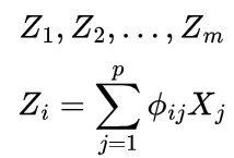
The linear regression problem then becomes

We have now successfully reduced the problem from p dimensions to m. Having found a principle to base our transformations on, we now briefly look at 3 ways to decide how to pick our new (transformed) predictors.

Principal Component Analysis (PCA) is a popular approach to derive a low dimensional set of features from a large set of features. It is based on the idea that the first principal component is that along which the observations vary the most. The rationale being that we are trying to capture the most information possible.

This is akin to finding a line as close as possible to the data, i.e. minimizing the RSS! The next direction must then be linearly independent to the first and so on.

An example of PCA. (Source : ISL Python)

In the above example, we consider the ad spending (in 1,000 $) of a company as a function of the population (in 10,000) of cities. The first plot shows the first principal component, i.e. the least squares fit. In this case it Z_1 = a * population + b * ad spending for some values (a,b). These values are called the principal component scores .The plot on the right rotates this so that the 1st principal component is along the x axis.

Since we have only two predictors we can have atmost 2 principal components, the second of which has to be perpendicular to the first.

With a way to reduce dimensions, we now need to fit linear regression on these new transformed variables. We discuss two ways of doing this (albeit briefly):

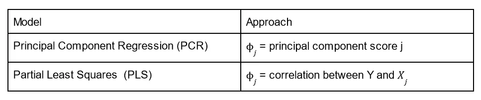
PCR works well when the variation in the data is captured in the first few principal components. But it has a draw back, while the transformed variables can express the predictors well, they don’t do well in predicting the response Y.

PLS tries to solve this issue by setting the coefficients of the linear combinations equal to the correlation b/w Y and X_j from simple linear regression.

This section was much shorter than the rest. It meant to serve as an introduction to a concept we will return to in chapter 12 : unsupervised learning, so stick along until then.

Conclusion

With all these methods in place, we can still come up short 😔 In general adding signal features that are truly associated with the response will help decrease the test error. But finding them out is where the challenge lies.

We need to remember 3 things to this end : (i) regularization or shrinkage plays a key role in high dimensional data (ii) appropriate parameter selection is crucial for good predictive performance (iii) in general the test error of the model increases with dimension.

With high dimensional data the multi-collinearity problem is extreme ; any variable can be written as a linear combination of other variables. Essentially, this means that we can never know which (if any) predictors influence the response and only hope to identify the best possible coefficients for regression.

In our DNA example even if we do arrive at a model with say 17 genes to predict a disease, we need to acknowledge that this is only one of several possible models whose results need to be validated on independent test sets.

Oh and the fancy RSS, R², p-value and other formulas we developed & applied to training data should never be used for high dimensional data. Always quantify your results using independent test sets :’)

P.S. This is my 10th blog post 🥳 It took 5 months to get here, and a 144 reads later I must reflect on how rewarding this entire process has been. From dreading writing for others (and dangerous deadlines) to understanding what I learn better, writing this blog has changed not only the depth of my knowledge but also my learning methods. To this end, I think it has helped me more than any of my readers.

It’s also appropriate to thank one special reader. They’ve read all my posts and given constructive feedback on each one (under no obligation whatsoever), improving not only the posts but my communication skills. Now each time I type a sentence, I think whether they would understand what I am putting across. Countless discussions (online and offline) with them have made me not only a better writer, but also a better person.

Thank you for everything my m&m ❤