Chapter 5: Resampling Methods

Having studied a few machine learning algorithms (for both regression and classification), we come back to the dreaded topic of evaluating their performance … which means tests !

In real life we almost never have access to unseen testing (validation) data. This means we need to predict how our model will perform on unseen data, using only our training data. These methods are called re-sampling since they involve repeatedly drawing samples from the training and fitting models on them.

In this post I will explain 4 re-sampling algorithms. In the figures below, the training set is shown in blue color and the validation set is shown in orange color.

50/50

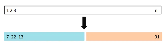Validation set approach. (Source : ISL Python)

In the validation set approach we randomly divide a data set with n points into two equal halves. We train the model on one half and test it on the other. Let’s see how this works in practice. We perform polynomial regression on quantitative data and find out mean squared error of our model as a function of the polynomial degree. We repeat this procedure for many validation set splits.

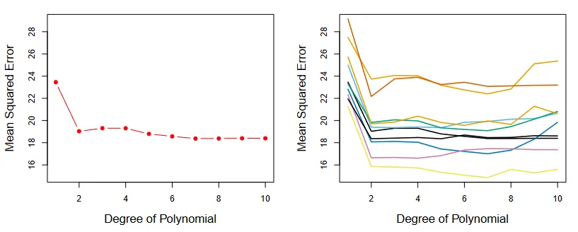Validation set results. (Source : ISL Python)

From the left hand plot it is clear that f is approximated best by a polynomial of degree 2. In the right hand side we see the results for various random splits, which confirm that a quadratic fit is the best.

But the right hand plot also reveals some problems. Different splits of the data cause different errors, which leads to estimates with high variability. Problems are made worse by the fact that we are training on the model on such a small subset of data, this leads to an overestimate of the validation error.

99/1

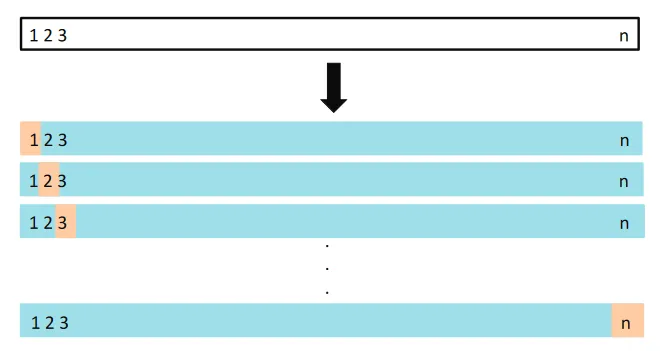LOOCV approach. (Source : ISL Python)

In the Leave One Out Cross Validation (LOOCV) approach we split the n data points into individual points. We train the data on n-1 points and test our prediction on the left over point, this gives us one mean-squared error. We repeat this process, making each point from the training data as the validation point. Averaging over all the errors, gives us the validation error.

Note that this is not a random process, and we systematically use each point as the validation point. We are doing better now, the variability in the validation error is now removed, owing to the fact that there is no randomness involved. Running LOOCV multiple times yields the same result. LOOCV also does not overestimate the validation error, owing to the large number of data points available for training.

There are some problems though. Fitting such a model is computationally expensive, especially as n grows. Another problem is that the training pints have a large positive correlation, since they only ever differ by one point each time, this leaves our estimate highly biased.

Fractions

K-folds approach. (Source : ISL Python)

The k-folds approach strikes a balance between variance(validation set) and bias(LOOCV), the equivalent of the point we want to reach in the bias-variance trade off. Not too unassuming, but not too specific either.

Here we randomly divide the n data points into k fractions, each with n/k points. Once this division is done, we train the model on k-1 sets and test in on the remaining one. We do this for each of the k splits and average their errors to estimate the validation error. Note that k-folds for k=n is the same as LOOCV.

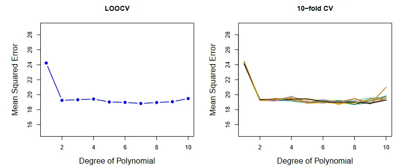K-folds results. (Source : ISL Python)

We see in the right hand panel, that we have very little variability. So k-folds strikes the balance between randomness and size of training data. By experiment it is found that k=5 and 10 give the best estimates for the validation error.

The Bootstrap

Bootstrap approach. (Source : ISL Python)

The Bootstrap is a method that applies to many situations other than just validation error estimation. In general, it is a good method to use when we want to estimate statistical quantities that do not have a simple closed form solution.

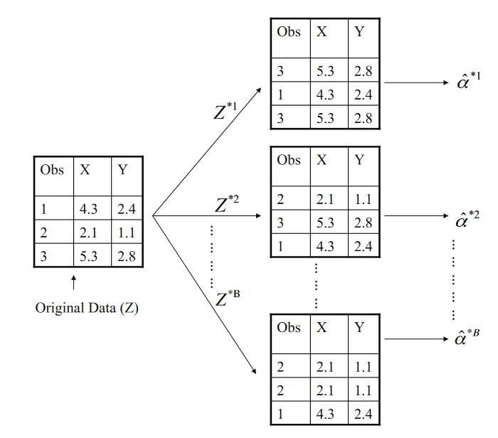
Assume we have a data set Z with 3 (n) points, bootstrap makes B sets of training examples Z*(i) , each of size 3 (n). These B sets form our training data, and we fit a model on each of them. The final estimate is given by averaging individual values.

The way that bootstrap makes a training example is the following, it picks a point randomly from the original data (each point having equal probability) and adds it to the example. Then it replaces this point and picks another point randomly, until the training example is of size 3 (n). This means that the same point can appear more than once (as shown in the above graphic).

The advantage of bootstrap is that it doesn’t make any assumptions while estimating statistical quantities, giving more reliable estimates. The drawback being computational cost.

While this post covered quantitative data, the same methods apply for qualitative data too. In that case errors take on values of 1/0 based on classification/misclassification.

This chapter was more theoretical than the rest and introduced some algorithms too. While it’s easy to assume you understand them, I urge you to code the logic for the ones discussed here yourself (yes, I mean don’t use another library). Doing that myself revealed gaps in my knowledge and forced me to write the logic line by line, till the computer executed exactly what I had in mind.