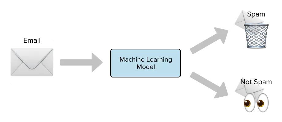Classifying email as spam or ham

In the last chapter we dealt with response variables that were quantitative, and tried to predict a numerical quantity. But in many situations the response variable is qualitative, (i) email is spam/not (ii) person has disease/not (iii) stock will move up/down (iv) image of dog/cat and so on. In this setting we assign each data point to one category. This process is called classification.

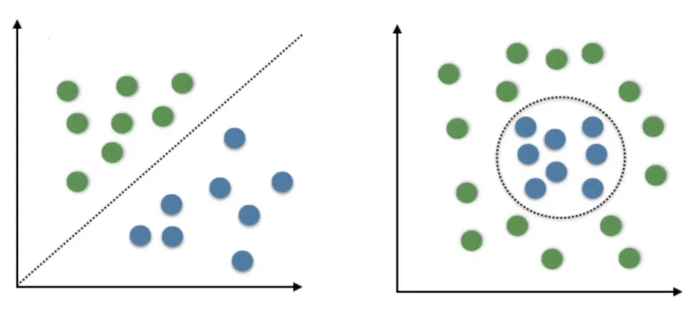Examples of Classification Problems. (Source : Naukri.com)

In the above graphic we see a simple 2-D example of classification. We see data points of two different classes, blue and green. In the first case, a straight line is enough to separate them ; anything to the left of the line is classified as green. In the second case, we need a circle for clear separation. The line and the circle are called as the decision boundary.

The important assumption here being that we can separate the different classes !

What about Linear Regression ?Permalink

We saw that linear regression was capable of handling qualitative variables by making a dummy variable that took values 0/1 indicating the absence/presence of a qualitative variable. Why then do we need new algorithms ?

We make predictions for classification using probabilities, that is if a particular observation X = x has a probability p of belonging to a certain class Y = k that is above some predefined threshold, we classify it as belonging to class k.

Here we see the first problem with linear regression. It can predict negative probabilities, since intercepts for straight lines can often be below 0. As we increase x, the probability increases, surpassing 1. Hence p ∉ [0,1] in the case of linear regression, disqualifying it.

Another reason is that when we have more than 2 classes, ordering them can lead to problems if there is no ascending/descending order. Take for example trying to diagnose a patient based on their systems using linear regression.

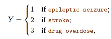
Multi-class dummy variable. (Source : ISL Python)

In the above example there is no particular reason that stroke is in position #2 and drug overdose #3. A different encoding can lead to different inferences. We also have no reason for the difference b/w the three diseases to be the same (1 in this case).

Hence we see that for more than 2 classes, there is no meaningful way to perform linear regression for classification. So the hunt is on for functions that give outputs ∈ [0,1] for any & all inputs.

Logistic regressionPermalink

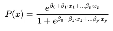
One such model is logistic regression, which has the following functional form. We notice that the log odds i.e. log (p/1-p) is linear in x.

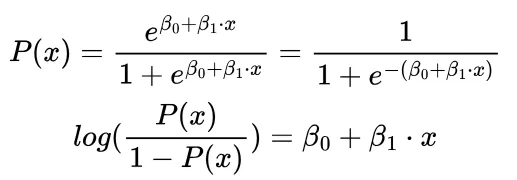
Why is this a reasonable function ? For small values of x, when x=0 we see that p becomes very small and approaches 0. For large values of x, when x → ∞ the exponential term disappears and p becomes 1. This gives the function a characteristic S shape. Let’s see how this looks in comparison to linear regression, trying to find credit card defaulters from bank balance.

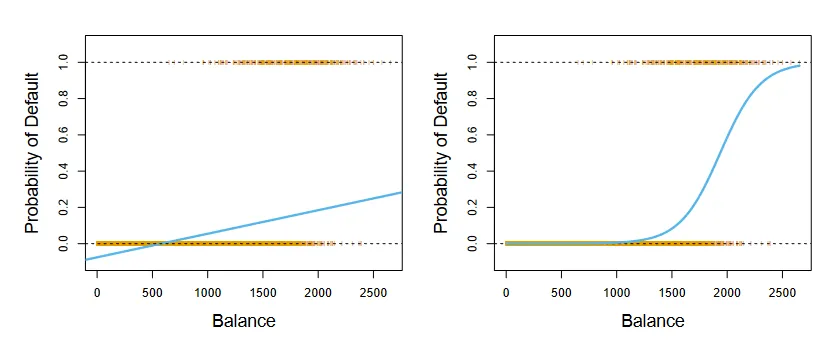Linear v/s Logistic regression curves. (Source : ISL Python)

The interpretation of the coefficients remains similar to linear regression. However increasing x by one unit increases the log odds by β1, we need to be careful about this subtlety. Regardless of this, a positive value of β is associated with an increase in p while a negative value of β is associated with a decrease in p.

The way we estimate the coefficients differs from linear regression. Here we want to maximize the probability of making a correct decision, which is encapsulated in a likelihood function. Below is an example of a simple likelihood function for binary classification.

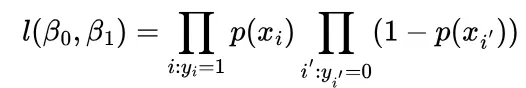
We (the computers) compute this value for all combinations of β and pick the ones that maximize this value. Similar to linear regression we can also perform multiple logistic regression, which can reveal details hidden when performing simple logistic regression.

For the same example as before, we consider students(orange) and non-students(blue) as another predictor along with balance.

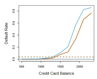
Multiple logistic regression. (Source : ISL Python)

It is clear that for a given balance, students tend to default lesser than non-students.

With the coefficient estimates in place, all that is left to do is make predictions and assign to a particular category. To compute the probability of a particular point we simply plug in the value of x into our model. A typical threshold for classification is p = 0.5, i.e. if the probability of default for a certain balance (and other features) is more than 0.5 then we predict that the person will default.

We rinse and repeat for all the data points and have successfully classified the entire data set !

A sample decision boundary. (Source : ISL Python)

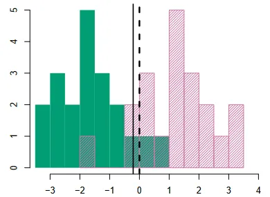
In the above graphic, we see a histogram of points (x,y) in a data set. At each value of x, we count the number of y values that equal green and pink, the count forms the height of the bar and the color of the bar indicates the class.

The Bayes’ boundary (best we can do) is shown by the dashed line. The boundary obtained in practice is shown by the solid line. All points to the left are classified as belonging to the green class, and to the right as belonging to the pink class.

Generative models & Bayes’ TheoremPermalink

Another way to find the probability of a data point belonging to a certain class is Bayes’ Theorem.

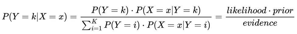Bayes‘ Theorem

In the above formula, the likelihood is easy to estimate as it is simply the fraction of training responses belonging to class k. The difficulty lies in estimating the prior. Once we have all the prior probabilities, computing the evidence is trivial. To find this prior, we need to make some assumptions about the form of the data. Let’s look at three models and the assumptions that they make.

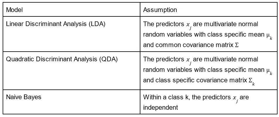
Once we pick a certain model and make certain assumptions about the data, we substitute the resulting formula in the equation for P(Y=k | X=x) and optimize for the values that give the highest likelihood. Each model leads to a new formula to optimize.

In practice we do not know the type of relation that exists in between the predictors and the classes, and hence it is difficult to compare the different models objectively and even decide which one is most suited for the problem at hand.

In general however if the true decision boundary is linear we expect logistic regression and LDA to perform well. When the boundaries are moderately non-linear, QDA or Naive Bayes might be better. For much more complicated decision boundaries, a non parametric approach like K nearest neighbors can be superior.

With all these models in place, we need a common metric to compare their performances. We need to understand the type of errors that our model is making, which can be understood using a confusion matrix. The ROC curve gives a visual representation of the two types of errors that a classifier can make.

It’s important to note that optimizing the classifier depends on the task at hand and requires domain knowledge. This means optimizing the model for either false positive / false negative performance.

Poisson RegressionPermalink

Finally, an interesting model to consider is Poisson regression. The Poisson model is used when we are dealing with counts.

Considering the problem of predicting the number of bicycles that a company rents out as a function of the season and also time of day.

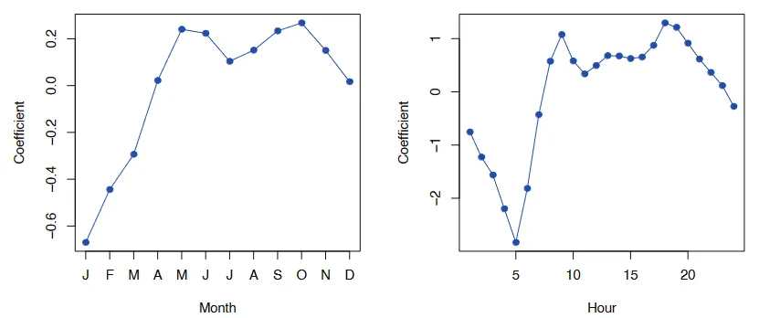Bicycles rented as a function of month & time of day. (Source : ISL Python)

The plot seems to be intuitive. During winter months & summer vacation nobody seems to be riding bicycles, and within a day the bicycles rented are most during commute times and lesser at other times. On first glance it seems that linear regression estimates can do a good job.

A closer look reveals it is not so. Like before linear regression still produces negative results, meaning negative bicycles rented ! Also we see that the variance in the number of bicycles rented changes with time and season (think 2 am on a January night v/s 9 am on a March morning), and linear regression is ill equipped to handle this. This is where Poisson regression shines.

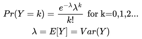
By definition this cannot produce negative numbers and we have found a way to account for the change in variability.

This was a first look at classification, an important machine learning problem. There are even more methods for this task, and we will explore them in a later chapter(s).