Chapter 3: Linear Regression

Trying to find the most “fitting” straight line

One of the most easy and intuitive guess about the relationship between data (X) and response (y) is the linearity assumption. The fare for your taxi increases linearly with the distance traveled, the salary you earn is proportional to the number of hours you work … and so on. Let’s see how this simple yet powerful algorithm works in machine learning.

Simple Linear Regression

We estimate y = f(X) + Ɛ by a straight line in this case, therefore y = mx + c. Where m is the slope (how steep the line is) and c is the intercept (the value of y when x=0).

But this is the general equation of a line, how do we know which one to pick ? That’s where calculus steps in. The goal is to find a a line where the squared distance (we don’t care if the point is above / below) of each point in X from that line is the least, in the figure below this is shown in grey.

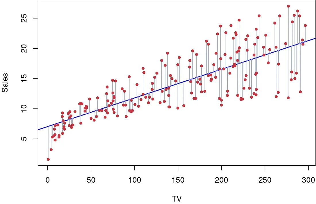Sales of a company as a function of TV advertisement budget. (Source : ISL Python)

To form an expression for this distance & to minimize it, let’s formulate exactly what we need.

So now all we need to do is minimize RSS with respect to both the intercept (β0) and the slope (β1) in order to form our straight line. To find the minimum values of the intercept & slope, we simply differentiate R_SS partially_ with respect to that particular variable & set it equal to 0. In the 1 dimensional case this has a simple solution … but with more dimensions things get real messy real quick, so we let the computers deal with the calculus !

Metrics for line & model evaluation

How do we know how close our straight line is to the straight line in question (if it exists)? How do we know well our straight line works on the data?

Before we start let’s acknowledge the Law of Large Numbers (LLN)which states that given enough trials, our estimates for the real value of a quantity will converge to that real quantity (if it exists). In our case, this means that a true slope & intercept can be found afterall.

Red is the true straight line, and blue is our estimate. (Source : ISL Python)

In the right hand panel we see the LLN play out. With repeated linear regression on different subsets of X (shown in light blue) we see our line get closer and closer to the true line in question. With confidence that we can achieve greatness, we now compute some statistical quantities.

Part (a) : goodness of straight line

The first of which is the standard error, a measure of how much one single estimate varies from the true value. Standard errors can be used to compute confidence intervals. A 95% confidence interval is interpreted as follows : if we take repeated samples and construct the confidence interval for each interval, then 95% of those intervals will contain the true value of the parameter we want to estimate.

Another thing that standard errors help us form are hypothesis tests, the most common of which is the null hypothesis. The null hypothesis is H0 : there is no relationship b/w X and y, which is tested against an alternate hypothesis Hα : there is some relationship b/w X and y. To test these hypotheses we compute t statistics & p values.

Where t-statistic = estimate for β / standard error of β. The t statistic measures the number of standard deviations that β is away from 0, hence a larger t-statistic is favorable. The p value is the probability of observing an association b/w X and y due to chance. The lower a p value, the more confidence we have in our straight line. Phew, with so many formulas in place we can finally see how good our line is.

Some numbers related to our straight line. (Source : ISL Python)

Since the p values are sufficiently small, we have made good estimates for the slope & intercept.

Part (b) : goodness of model

While we may have a good straight line, if our line doesn’t help explain the data, we aren’t doing any good. To see how well our line explains the actual functional form of the data, we need a new statistic.

Here ȳ is the mean value for y. The TSS represents the error in the model before we fit the linear regression model, checking how much each point varies from the mean. R² then is a measure of the proportion of variability in Y that is explained by our straight line. By definition R² is a number b/w 0 and 1, with a higher value being better (ideally we would have no RSS and R² would be 1 !).

By regressing Sales data onto TV advertising we get an R² value of 0.612, which means our model explains 60% of the variability in the data.

Multiple Linear Regression

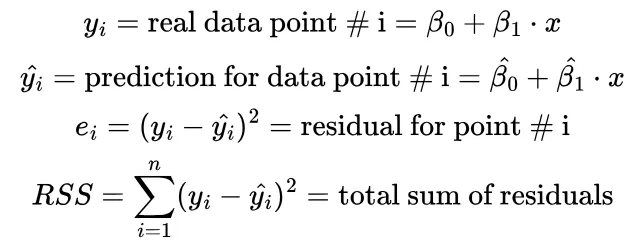
In most cases, data is not one dimensional and hence we need to include multiple predictors (Xi) in our quest to model the response (y). In 3-d we end up with a plane, and everything after is a hyperplane.

The goal of the algorithm still remains the same i.e. we want to reduce the distance of each point from our hyperplane. We also re-do the drills to compute the goodness of our estimates and the model itself.

We interpret the individual slopes as follows. β1 gives the unit increase in y per unit increase in x1, keeping all other predictors fixed.

A sample multiple linear regression estimate. (Source : ISL Python)

But why ever bother with multiple linear regression when I can do simple linear regression multiple times you ask? Well, this is because of correlation. Often times two predictors are related linearly, and simple linear regression can make it look like one of them is important when in actual fact it is not.

For example, consider regressing shark attacks onto ice cream sales at a beach over time. Simple linear regression would conclude that ice cream sales are associated with shark attacks ! But the reality is : increase in temperature → increase in people on the beach → increase in ice cream sales & shark attacks alike. Multiple linear regression shows that shark attacks depend on the temperature, and ice cream sales was just taking credit for being associated with rising temperatures ! Causal inference is a slippery slope to scale.

Moving beyond linearity

One problem with the multiple linear regression model we saw above was that each predictor (Xi) was assumed to be independent of the other. This is often not the case since predictors depend on each other. One way to tackle this is to add interaction terms (a product / combination of predictors).

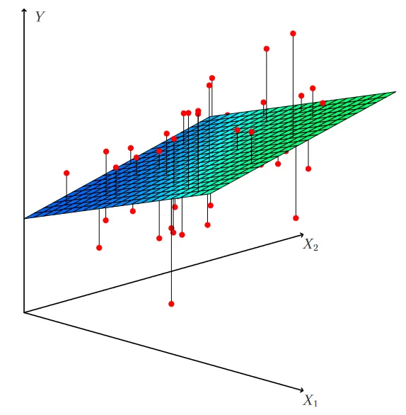
Consider a model for predicting bank balance based on income for students and non-students, full with interaction terms like (β1+β3)*income.

We see that the slope and intercepts change based on whether the person in question is a student or not, a fairly reasonable estimate to make.

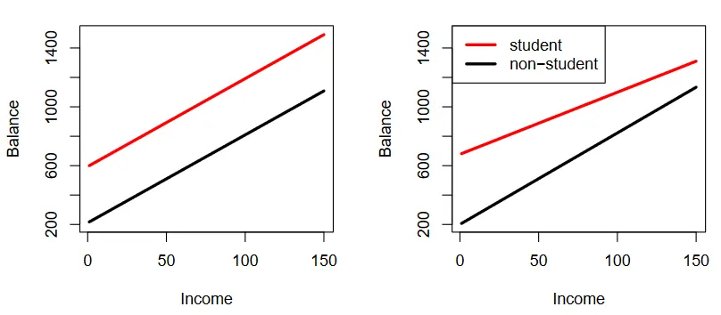The difference in models with & without interaction terms. (Source : ISL Python)

The lines on the left have no interaction terms whilst the right hand panel includes an interaction term, making a considerable difference (it seems students step up their balance much slower 😅).

We can also add higher powers of the predictor to better fit the data. This is called polynomial regression.

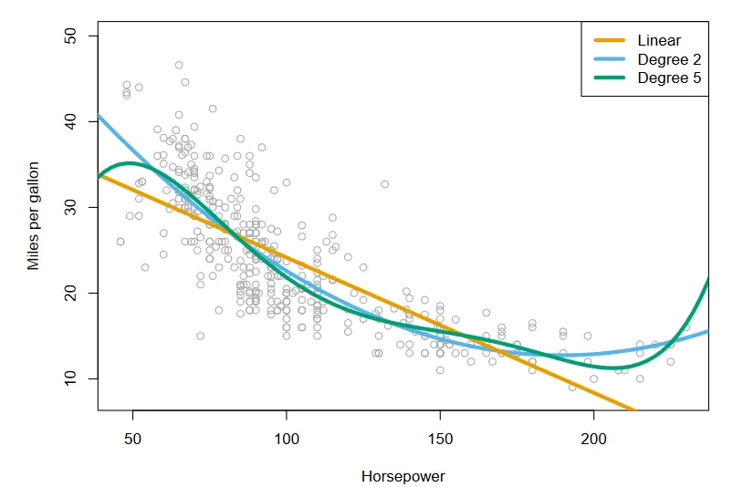Polynomial regression on data related to cars. (Source : ISL Python)

Linear Regression is a fundamental machine learning algorithm, which is often a good place to start when analyzing data. Many other algorithms can also be considered an extension of the linear model. While this post gives a broad introduction to the topic, a lot of the content from the textbook (66 pages chapter) was omitted here. I would strongly suggest reading the textbook for a deeper understanding.

For understanding the statistics involved a few resources that have helped me are : zstatistics and seeing theory.