Chapter 2: Statistical Learning

From detecting heart disease in medical images to recommending the next show you should binge watch, machine learning is everywhere. But what exactly is machine learning ? How does it work and what can it do ? In this post I try and answer some of those questions.

What is statistical (machine) learning ?

Machine learning is the development and study of algorithms that can learn from data and generalize to unseen data, and thus perform tasks without explicit instruction.

Let’s try to understand this with an example and phrase it in a more mathematical manner.

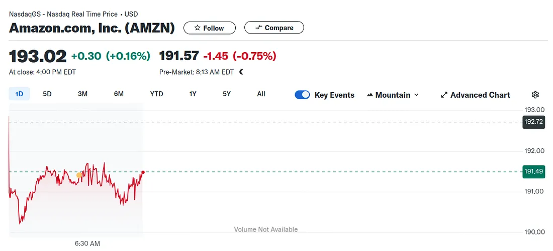The stock price of Amazon on 17 July, 2024. (Source :Yahoo finance)

In the image above we see the price change in price of the Amazon stock on July 14, 2024 as a function of time, volume of stocks traded, etc. Machine learning can be used here to predict the direction that the stock will move tomorrow. That is, will it increase in value or decrease ?

Another way to think about machine learning then is, using known inputs (volume of stocks traded, time of day) and known outputs (stock price), predict a future (unknown) output provided the same type of inputs.

Therein lies the essence of machine learning, “learning” from past data in order to predict future data.

The only assumption here is that : there exists some underlying relation between the inputs (say X) and outputs (say Y). If this relation is inherently random, no amount of machine learning yields meaningful results.

Where exactly is the learning you ask ? Assume that X and Y are related through some function f. The program of machine learning is to estimate f from known (training) data, test how well the estimate worked on unknown (testing) data and improve the estimate based on the result.

There’s just a slight caveat, which is : what do you want your machine learning model to do ? Do you want to predict Y given X or do you want to understand how X and Y are related ? This is the distinction between prediction and inference, something we will have to pay closer attention to..

How to estimate f ?

Let’s consider another (albeit simpler) example. Consider data on income as a function of years of experience (seniority) and levels of education. It seems intuitive that with high educational qualifications and more years on the job, you should be payed more.

But before we can start building a model, we need to ask ourselves : prediction or inference ? Let’s look at some data and see how our estimate for f might change in both cases.

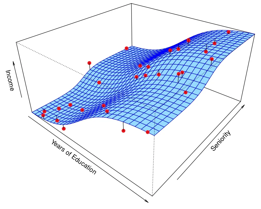A sample function f. (Source : ISL Python)

The data points are marked in red and the estimate f is the blue plane. The error between the prediction and real value is shown in the straight black line. While the relationship is largely linear, it is not entirely so. If we want to understand how years of education and seniority influence the income, we would estimate f to be a linear function, thereby missing some of the points. If we want to predict the income (Y) given years of education and seniority (X) we would account for some non-linearity. Both of those cases are shown below.

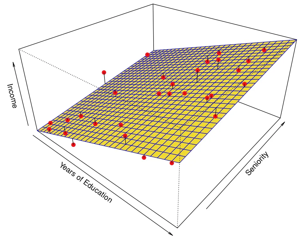Inference model. (Source : ISL Python)

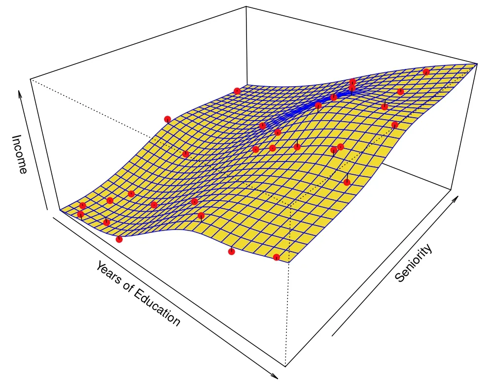Prediction model. (Source : ISL Python)

This is the trade off that we need to consider. In the inference case, there will be a larger error in between our estimate and the observed value. Whereas the error will be lower in the prediction case, at the cost of explainability. Ideally we hope to strike a balance between inference and prediction. This is called the model accuracy and interpretability trade off, and different models are good for different tasks.

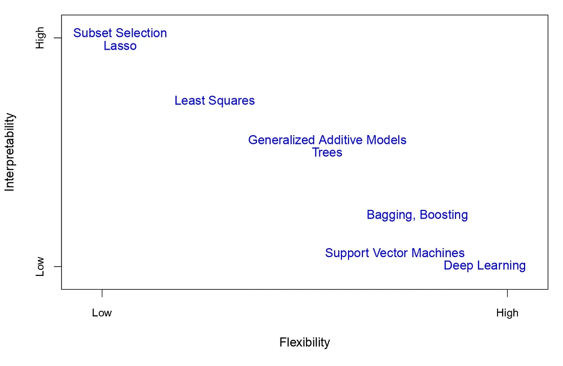The types of machine learning algorithms. (Source : ISL Python)

Types of machine learning

The first distinction comes from the nature of the data itself. Is it quantitative (numerical) or qualitative (non numerical) ? Numerical data leads to regression problems and non-numerical data leads to classification problems. For instance, predicting house prices based on various aspects (number of rooms, size of kitchen, etc..) is a regression problem while checking if an email is spam or not is a classification problem.

Another distinction comes from whether or not the data is complete. If we have access to both X (inputs) and Y (outputs) it is called as supervised learning. An example of which is the income example we saw above. If however all we have access to is X without direct information about Y, then it is unsupervised learning. An example of this is clustering customers on amazon as big spenders or small spenders based on information on amounts spent and purchase frequency.

How well am I learning ?

This image was generated using Meta AI

While studying a course in school, the metrics used to measure a students understanding are tests. Likewise, to test the working of our model, we have it sit a test.

In the case of machine learning, this means making predictions about unseen Y (outputs) using past experience and evaluating performance after a subsequent measurement Y’. Just like how doing well on homework throughout the school year (learning process) doesn’t matter in the face of the final exam, a model’s training accuracy is only secondary (if at all relevant) in comparison to testing accuracy.

This leads to a slight modification to our model accuracy and interpretability trade off. We now need to deal with the bias and variance trade off. Here bias represents the error in estimating the nature of f . For example, if the data is highly non-linear and our model is linear, the model has a large bias. Variance represents the error in our model if we change the data set slightly. For example, if our model is non-linear adding or removing a single data point makes a significant change to f, we say the model has a large variance.

Like with our previous trade off, we want to find a balance between the bias and variance of our model. If we fit out data very loosely, we risk under-fitting, completely ignoring the relation between X and Y. If we fit our data too close, we risk over-fitting, finding relationships that don’t exists in the first place.

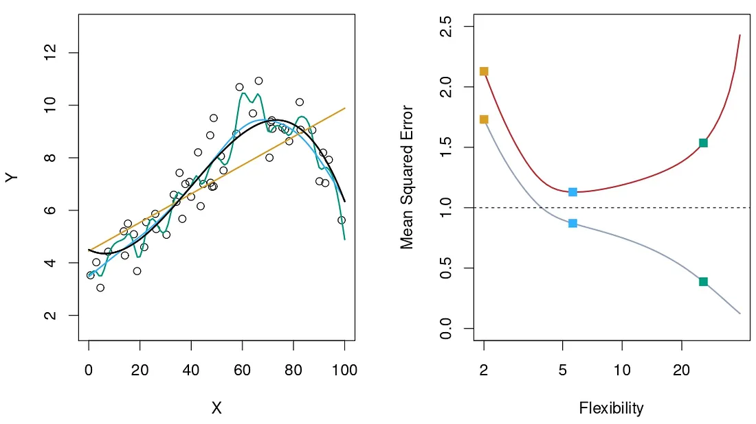An example of different models and their error. (Source : ISL Python)

In the plot to the left, the black line indicates the real function f, the yellow line is a linear fit, the blue is slightly non-linear and the green is high non-linear. The plot on the right shows the errors ( training error = grey, testing error = orange ) as a function of the model’s flexibility. The yellow square is a case of under-fitting, the green is a case of over-fitting. Blue is what we aim at.

This is a broad introduction to machine learning, it’s nature and it’s scope. This (and the subsequent) post(s) is based on the book An Introduction to Statistical Learning with Applications in Python. I am working through the book and will summarize each chapter in the form of a blog post (hopefully once a week). My solutions to the exercises can be found here. I hope you understand machine learning a little better than when you started reading !